Unsupervised Hierarchical Symbolic Regression for Interpretable Property Modeling in Complex Multi-Variable Systems
英文原文与中文译文逐段对照 · English original with Chinese translation
Siyu Lou ${}^{1,2}$ D | Chengchun Liu ${}^{3}$ D | Dongxiao Zhang ${}^{2}$ | Yuntian Chen ${}^{2}$ D | Fanyang Mo ${}^{3,4,5,6}$
楼思雨${}^{1,2}$ D | 刘丞军${}^{3}$ D | 张东晓${}^{2}$ | 陈云天${}^{2}$ D | 莫凡洋${}^{3,4,5,6}$
${}^{1}$ School of computer science, Shanghai Jiao Tong University, Shanghai, P.R. China ${}^{1}{}^{2}$ Ningbo Key Laboratory of Advanced Manufacturing Simulation, Eastern Institute of Technology, Ningbo, P.R. China I ${}^{3}$ School of Materials Science and Engineering, Peking University, Beijing, P.R. China I ${}^{4}$ School of Advanced Materials, Peking University Shenzhen Graduate School, Shenzhen, P.R. China I ${}^{5}$ AI for Science (AI4S)-Preferred Program, Peking University Shenzhen Graduate School, Shenzhen, P.R. China I ${}^{6}$ Guangdong Provincial Key Laboratory of Nano-Micro Materials Research, Peking University Shenzhen Graduate School, Shenzhen, P.R. China
${}^{1}$ 上海交通大学计算机科学学院,上海,中国 | ${}^{1}{}^{2}$ 宁波先进制造仿真重点实验室,东方理工学院,宁波,中国 | ${}^{3}$ 北京大学材料科学与工程学院,北京,中国 | ${}^{4}$ 北京大学深圳研究生院先进材料学院,深圳,中国 | ${}^{5}$ 北京大学深圳研究生院人工智能促进科学(AI4S)优先计划,深圳,中国 | ${}^{6}$ 广东省纳米微材料研究重点实验室,北京大学深圳研究生院,深圳,中国
Correspondence: Yuntian Chen () | Fanyang Mo ()
通信作者:陈云天 () | 莫凡洋 ()
Received: 23 October 2025 | Revised: 15 December 2025 | Accepted: 19 December 2025
收到日期:2025年10月23日 | 修订日期:2025年12月15日 | 接受日期:2025年12月19日
Keywords: explainable AI | molecular polarity | molecular structure | symbolic regression | TLC
关键词:可解释人工智能 | 分子极性 | 分子结构 | 符号回归 | 薄层色谱法
ABSTRACT
摘要
Recent advances in artificial intelligence have produced powerful predictive models for chemical analysis, but model interpretability remains a challenge. Here, we introduce Unsupervised Hierarchical Symbolic Regression (UHSR), providing an explainable solution while maintaining competitive predictive performance. With a focus on thin-layer chromatography (TLC), a crucial technique in molecular polarity analysis, UHSR automatically distills chemically-intuitive retention indices and discovers explainable equations that link molecular structures to chromatographic behavior. Experiments have shown UHSR’s capability to derive concise and accurate governing equations linking polarity to molecular structures from the TLC dataset. A survey of 100 expert chemists demonstrates that our UHSR model gains more trust from chemists compared to traditional models. Additionally, we also show its adaptability to other property prediction tasks beyond molecular polarity.
人工智能的最新进展为化学分析产生了强大的预测模型,但模型的可解释性仍然是一个挑战。在这里,我们引入了无监督分层符号回归(UHSR),在保持有竞争力的预测性能的同时提供了一个可解释的解决方案。以薄层色谱法(TLC)为重点,这是分子极性分析中的一项关键技术,UHSR自动提取化学直观的保留指数,并发现将分子结构与色谱行为联系起来的可解释方程。实验表明,UHSR能够从TLC数据集中导出将极性与分子结构联系起来的简洁准确的控制方程。对100位化学家专家的调查表明,与传统模型相比,我们的UHSR模型获得了化学家更多的信任。此外,我们还展示了它对分子极性以外的其他性质预测任务的适应性。
1 | Introduction
1 | 引言
Scientific discoveries aim to explore and understand the world through the observation of phenomena, the systematic collection of data, the identification of patterns, and the elucidation of underlying principles that enable the prediction of future events [1, 2]. The derivation of empirical equations and parameters through data-driven methods has been pivotal in elucidating chemical phenomena and predicting experimental outcomes. For example, Henry’s Law $\left( {C = {k}_{H} \cdot P}\right)$ for solubility predictions [3], the Arrhenius equation $\left( {k = A \cdot {e}^{-\frac{{E}_{a}}{RT}}}\right)$ for reaction rate dependence on temperature [4], and the van’t Hoff equation
科学发现旨在通过对现象的观察、数据的系统收集、模式的识别以及对能够预测未来事件的潜在原理的阐明来探索和理解世界[1,2]。通过数据驱动方法推导经验方程和参数在阐明化学现象和预测实验结果方面一直起着关键作用。例如,用于溶解度预测的亨利定律$\left( {C = {k}_{H} \cdot P}\right)$[3],用于反应速率对温度依赖性的阿仑尼乌斯方程$\left( {k = A \cdot {e}^{-\frac{{E}_{a}}{RT}}}\right)$[4],以及范特霍夫方程
This is an open access article under the terms of the Creative Commons Attribution License, which cited. $\left( {\ln K = - \frac{\Delta {H}^{ \circ }}{RT} + \frac{\Delta {S}^{ \circ }}{R}}\right)$ for equilibrium constants related to temperature [5]. These empirical equations and parameters, derived through extensive experimental work and large datasets, remain foundational in contemporary chemistry.
这是一篇根据知识共享署名许可协议条款发布的开放获取文章,该协议已被引用。$\left( {\ln K = - \frac{\Delta {H}^{ \circ }}{RT} + \frac{\Delta {S}^{ \circ }}{R}}\right)$用于与温度相关的平衡常数[5]。这些通过大量实验工作和大型数据集推导出来的经验方程和参数,在当代化学中仍然是基础。
Polarity, reflecting the uniformity and symmetry of charge distributions in molecules, is crucial for understanding molecular interactions and characterizing molecules $\left\lbrack {6,7}\right\rbrack$ . Chromatography serves as an essential tool for studying polarity by providing insights into how molecules interact under various chemical environments. Over the years, various chromatographic models have been developed to describe retention behavior and polarity-driven interactions. For example, linear free energy relationship models [8, 9] have focused on analyte-stationary phase interactions, capturing how polarity influences adsorption and desorption processes. Similarly, solvent strength models [10, 11] have been widely used in reversed-phase liquid chromatography. These models are explicitly designed for binary aqueous-organic systems, where polarity differences between water and organic solvents are key drivers of retention behavior.
极性反映了分子中电荷分布的均匀性和对称性,对于理解分子间相互作用和表征分子$\left\lbrack {6,7}\right\rbrack$至关重要。色谱法是研究极性的重要工具,它能深入了解分子在各种化学环境中的相互作用。多年来,已经开发了各种色谱模型来描述保留行为和极性驱动的相互作用。例如,线性自由能关系模型[8,9]专注于分析物与固定相之间的相互作用,捕捉极性如何影响吸附和解吸过程。同样,溶剂强度模型[10,11]已广泛应用于反相液相色谱。这些模型明确设计用于二元水 - 有机系统,其中水和有机溶剂之间的极性差异是保留行为的关键驱动因素。
Siyu Lou and ChengChun Liu contributed equally to this work.
娄思宇和刘丞军对本工作贡献相同。
Thin-layer chromatography (TLC) provides critical insights into the behavior of organic molecules in various organic solvent environments. Polarity is a key factor in TLC, as the interactions between solutes, solvents, and the stationary phase are largely governed by differences in polar and nonpolar characteristics. However, TLC is usually labor-intensive and involves many repetitive trials [12, 13]. Despite its importance in determining the retardation factor $\left( {R}_{f}\right)$ , previous prediction models for structure-retardation factors have been limited by the quantity and standardization of TLC data [14, 15]. To address this challenge, our prior work introduced an automatic high-throughput platform for TLC analysis, providing a more extensive and standardized dataset for model training [16, 17]. This enhanced dataset not only improves the performance of predictive models, enabling more accurate and robust predictions of structure-retardation factors in TLC experiments, but also facilitates a better analysis of the liquid-liquid interactions between solutes and solvents.
薄层色谱(TLC)为了解有机分子在各种有机溶剂环境中的行为提供了关键见解。极性是TLC中的一个关键因素,因为溶质、溶剂和固定相之间的相互作用很大程度上由极性和非极性特征的差异决定。然而,TLC通常劳动强度大,涉及许多重复试验[12,13]。尽管其在确定阻滞因子$\left( {R}_{f}\right)$方面很重要,但以前的结构 - 阻滞因子预测模型受到TLC数据的数量和标准化的限制[14,15]。为了应对这一挑战,我们之前的工作引入了一个用于TLC分析的自动高通量平台,为模型训练提供了更广泛和标准化的数据集[16,17]。这个增强的数据集不仅提高了预测模型的性能,能够在TLC实验中更准确、更可靠地预测结构 - 阻滞因子,还便于更好地分析溶质和溶剂之间的液 - 液相互作用。
In recent years, significant progress has been made in artificial intelligence (AI)-assisted chemical analysis, especially in the development of quantitative structure-activity relationships (QSAR) prediction models [18-22] and quantitative structure-property relationships (QSPR) prediction models [23-25]. While these models have achieved remarkable prediction accuracy, the AI models and feature representations they employed often lack interpretability, hindering a deeper understanding of the underlying relationships within the dataset.
近年来,人工智能(AI)辅助化学分析取得了重大进展,特别是在定量构效关系(QSAR)预测模型[18 - 22]和定量构性关系(QSPR)预测模型[23 - 25]的开发方面。虽然这些模型取得了显著的预测准确性,但它们所采用的AI模型和特征表示往往缺乏可解释性,阻碍了对数据集中潜在关系的更深入理解。
The lack of transparency not only restricts the scientific impact of these models, but also undermines researchers’ ability to fully trust and understand their predictions [26-28]. To address this concern, there is an increasing need for (1) transparent models and (2) interpretable feature representations that not only achieve high performance but also align with human reasoning and provide meaningful insights.
缺乏透明度不仅限制了这些模型的科学影响力,还削弱了研究人员完全信任和理解其预测的能力[26 - 28]。为了解决这一问题,越来越需要(1)透明模型和(2)可解释的特征表示,这些表示不仅要实现高性能,还要与人类推理一致并提供有意义的见解。
One strategy to build transparent models is to articulate explicit formulas between the ${R}_{f}$ values and the solute molecular structures as well as the eluent solvents in TLC analysis. Symbolic regression (SR) has recently emerged as an effective approach for unveiling complex relationships within datasets [29-33], and has significantly contributed to many scientific discoveries [34- 40]. However, applying symbolic regression to datasets with a large number of variables remains challenging, as increasing the number of variables often leads to decreased performance and overly complex formulas, which undermines interpretability. For example, as shown in Supporting Information, when symbolic regression is directly applied to commonly used feature sets, such as physicochemical descriptors, the resulting models have limited predictive performance and reduced interpretability due to the high dimensionality. In terms of feature representations, molecular fingerprints, such as MACCS key molecular fingerprints [41], have been often used in AI models. However, these representations are typically high-dimensional and lack interpretability, making it difficult to understand how specific molecular structures influence the model prediction.
构建透明模型的一种策略是在TLC分析中明确阐述${R}_{f}$值与溶质分子结构以及洗脱剂溶剂之间的明确公式。符号回归(SR)最近已成为揭示数据集中复杂关系的有效方法[29 - 33],并为许多科学发现做出了重大贡献[34 - 40]。然而,将符号回归应用于具有大量变量的数据集仍然具有挑战性,因为变量数量的增加通常会导致性能下降和公式过于复杂,从而损害了可解释性。例如,如支持信息中所示,当将符号回归直接应用于常用的特征集,如物理化学描述符时,由于高维度,所得模型的预测性能有限且可解释性降低。在特征表示方面,分子指纹,如MACCS键分子指纹[41],经常用于人工智能模型。然而,这些表示通常是高维的且缺乏可解释性,使得难以理解特定分子结构如何影响模型预测。
In this work, we present unsupervised hierarchical symbolic regression (UHSR) (see Figure 1), a new SR approach guided by modular neural networks. UHSR introduces novel retention indices, e.g., solvent retention index and solute retention index, which are learned through a modular neural network. Guided by domain knowledge, this model comprises multiple sub-models that govern the mapping relationships between a set of input variables, e.g., solvent compositions, and a specific retention index, e.g., solvent retention index, as well as the mapping between retention indices and the output variable ${R}_{f}$ . It is noteworthy that this process aligns with the chemists’ thinking processes. The human brain struggles with high-dimensional information, opting not to directly comprehend intricate mappings but rather to decompose and analyze through individual sub-models. Then, we can apply the SR method on the output ${R}_{f}$ and the retention indices, effectively reducing the dimension of the input variables of the SR algorithm. Our experiments on the TLC benchmark dataset [17] demonstrate that UHSR achieves competitive prediction performance comparable to DNNs while providing concise formulas linking the ${R}_{f}$ value (indicative of the molecular polarity) with molecular structure features. Importantly, the retention indices and governing equations are evaluated by expert chemists, highlighting the alignment between the decision-making process of UHSR and that of chemists. Additionally, we extend the scope of our study to other chemical property prediction tasks, such as spectra-property prediction [42], where our framework also demonstrates high predictive accuracy and interpretability.
在这项工作中,我们提出了无监督分层符号回归(UHSR)(见图1),这是一种由模块化神经网络引导的新的SR方法。UHSR引入了新的保留指数,例如溶剂保留指数和溶质保留指数,这些指数是通过模块化神经网络学习得到的。在领域知识的指导下,该模型由多个子模型组成,这些子模型控制一组输入变量(例如溶剂组成)与特定保留指数(例如溶剂保留指数)之间的映射关系,以及保留指数与输出变量${R}_{f}$之间的映射关系。值得注意的是,这个过程与化学家思考过程一致。人类大脑难以处理高维信息,选择不直接理解复杂的映射,而是通过各个子模型进行分解和分析。然后,我们可以在输出${R}_{f}$和保留指数上应用SR方法,有效地降低SR算法输入变量的维度。我们在TLC基准数据集[17]上的实验表明,UHSR实现了与深度神经网络相当的具有竞争力的预测性能,同时提供了将${R}_{f}$值(指示分子极性)与分子结构特征联系起来的简洁公式。重要的是,保留指数和控制方程由专业化学家评估,突出了UHSR决策过程与化学家决策过程的一致性。此外,我们将研究范围扩展到其他化学性质预测任务,如光谱 - 性质预测[42],在这些任务中我们的框架也展示了高预测准确性和可解释性。
2 | Results
2 | 结果
2.1 | Data-Driven Explainable Retention Indices
2.1 | 数据驱动的可解释保留指数
It is essential for chemists to accurately characterize the overall polarity of molecules, as polarity influences molecular interaction, solubility, and chromatographic behavior. For this purpose, there are many known descriptors, such as the molecular polarity index (MPI), which is based on theoretical calculations. While effective in some cases, these descriptors have some limitations. For example, they are usually computationally expensive, especially for large or complex molecules. Also, they typically provide only global polarity information, failing to capture the localized effects of individual functional groups or their specific contributions to intermolecular interactions. Another way to estimate the molecule’s polarity is based on TLC experiments. This technique directly measures the ${R}_{f}$ value, which reflects how a molecule interacts with both the stationary and the mobile phase under specific experimental conditions. TLC experiments are relatively simple, low-cost, and widely accessible compared to computational methods, which often require advanced software, high-performance computing resources, and expert knowledge. By varying the solute or solvent composition and evaluating the resulting ${R}_{f}$ values, chemists can systematically study polarity in a way that is directly applicable to experimental workflows. Building on the strengths of TLC as a practical and experimentally grounded approach to studying molecular polarity, we identified several limitations in traditional methods of analyzing TLC data, which motivated this study. While TLC experiments provide valuable ${R}_{f}$ values that reflect molecular polarity, these raw experimental outputs are often difficult to interpret quantitatively and lack the ability to systematically separate solvent and solute contributions to retention behavior. Therefore, we developed a data-driven method to further refine the analysis. Using the TLC dataset, we extract two retention indices, namely $\Psi$ and $\xi$ , acting as empirical descriptors providing information about the polarity of the solvent system and the solute molecule, respectively. The clear chemical differentiation between solutes and solvents, alongside their near-zero Spearman correlation, compellingly validates our statistical methodology, as detailed in the Figure S1.
对于化学家来说,准确表征分子的整体极性至关重要,因为极性会影响分子间相互作用、溶解度和色谱行为。为此,有许多已知的描述符,例如基于理论计算的分子极性指数(MPI)。虽然这些描述符在某些情况下有效,但也存在一些局限性。例如,它们通常计算成本很高,尤其是对于大分子或复杂分子。此外,它们通常只提供全局极性信息,无法捕捉单个官能团的局部效应或它们对分子间相互作用的具体贡献。另一种估计分子极性的方法是基于薄层色谱(TLC)实验。该技术直接测量${R}_{f}$值,它反映了分子在特定实验条件下与固定相和流动相的相互作用方式。与通常需要先进软件、高性能计算资源和专业知识的计算方法相比,TLC实验相对简单、成本低且易于进行。通过改变溶质或溶剂组成并评估所得的${R}_{f}$值,化学家可以以一种直接适用于实验工作流程的方式系统地研究极性。基于TLC作为研究分子极性的实用且基于实验的方法的优势,我们发现了传统TLC数据分析方法中的几个局限性,这激发了本研究。虽然TLC实验提供了反映分子极性的有价值的${R}_{f}$值,但这些原始实验输出通常难以进行定量解释,并且缺乏系统分离溶剂和溶质对保留行为贡献的能力。因此,我们开发了一种数据驱动的方法来进一步完善分析。使用TLC数据集,我们提取了两个保留指数,即$\Psi$和$\xi$,分别作为提供有关溶剂系统和溶质分子极性信息的经验描述符。溶质和溶剂之间明显的化学差异以及它们近乎零的斯皮尔曼相关性,有力地验证了我们的统计方法,如图S1所示。
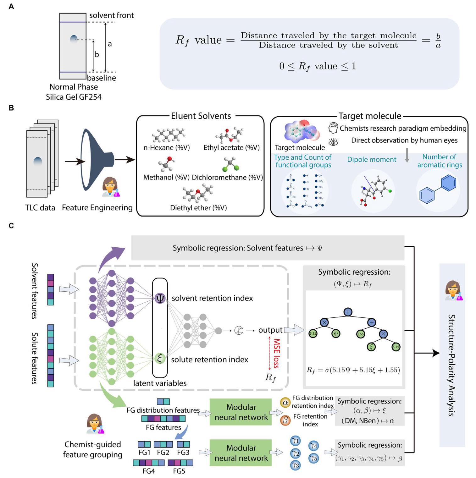
FIGURE 1 | Overview of Unsupervised Hierarchical Symbolic Regression (UHSR). (A) Illustration of TLC experiment and the calculation of the retardation factor $\left( {R}_{f}\right)$ . (B) Feature engineering, involving five solvent features based on volume percentages and the decomposition of target molecules into functional groups (FGs). The molecular structure is treated as a composite formed by stacking various functional group modules. (C) UHSR framework with three main stages: chemist-guided feature grouping, modular neural network for latent variable extraction (e.g., solute retention index $\xi$ ), and symbolic regression for discovering explicit equations between the target value and latent variables.
图1 | 无监督分层符号回归(UHSR)概述。(A)TLC实验及阻滞因子$\left( {R}_{f}\right)$计算的示意图。(B)特征工程,涉及基于体积百分比的五个溶剂特征以及将目标分子分解为官能团(FGs)。分子结构被视为由各种官能团模块堆叠形成的复合物。(C)UHSR框架,包括三个主要阶段:化学家指导的特征分组、用于提取潜在变量的模块化神经网络(例如溶质保留指数$\xi$)以及用于发现目标值与潜在变量之间显式方程的符号回归。
Importantly, compared to traditional physicochemical descriptors, our proposed indices are directly rooted in the experimental TLC dataset, which ensures that these indices are reflective of real-world molecular interactions. Furthermore, $\xi$ provides a localized and detailed perspective on molecular polarity, e.g., how specific functional groups impact the polarity through their specific contributions to solute-solvent and solute-stationary phase interactions. This detailed resolution allows $\xi$ to capture subtle variations in polarity that are often overlooked or averaged out by traditional global descriptors.
重要的是,与传统的物理化学描述符相比,我们提出的指数直接源于实验TLC数据集,这确保了这些指数反映了真实世界的分子相互作用。此外,$\xi$提供了关于分子极性的局部和详细视角,例如特定官能团如何通过它们对溶质 - 溶剂和溶质 - 固定相相互作用的特定贡献来影响极性。这种详细的分辨率使$\xi$能够捕捉到传统全局描述符经常忽略或平均掉的极性细微变化。
TABLE 1 | Description and statistical analysis of the features used in this study. The abbreviations, descriptions, mean values, along with the standard deviations (Std.), are presented. Additionally, Pearson’s correlation coefficients (r) are computed to quantify the linear relationship between each feature and the observed ${R}_{f}$ value.
表1 | 本研究中使用的特征的描述和统计分析。列出了缩写、描述、平均值以及标准偏差(Std.)。此外,计算了皮尔逊相关系数(r)以量化每个特征与观察到的${R}_{f}$值之间的线性关系。
| Abbreviations | Description | Mean(Std.) | Pearson's r |
| Eluent solvent | |||
| Hex | $n$ -Hexane concentration | 0.36(0.40) | -0.54 |
| EA | Ethyl acetate concentration | 0.15(0.28) | 0.29 |
| DCM | Dichloromethane concentration | 0.40(0.48) | 0.21 |
| MeOH | Methanol concentration | 0.014(0.025) | 0.31 |
| ${\mathrm{{Et}}}_{2}\mathrm{O}$ | Diethyl ether concentration | 0.071(0.22) | 0.13 |
| Solute molecule | |||
| NBen | Number of benzene ring | 1.12(0.57) | 0.07 |
| DM | Dipole moment | 1.34(0.74) | -0.02 |
| Ct Ph | Count of phenolic hydroxyl group | 0.15(0.40) | -0.15 |
| Ct ${}_{\mathrm{{OH}}}$ | Count of alcoholic hydroxyl group | 0.04(0.21) | -0.13 |
| ${\mathrm{{Ct}}}_{\mathrm{{Al}}}$ | Count of aldehyde group | 0.19(0.40) | -0.007 |
| ${\mathrm{{Ct}}}_{{\mathrm{{CO}}}_{2}\mathrm{H}}$ | Count of carboxylic acid group | 0.03(0.18) | -0.17 |
| ${\mathrm{{Ct}}}_{{\mathrm{{RCO}}}_{2}\mathrm{R}}$ | Count of ester group | 0.10(0.32) | 0.03 |
| ${\mathrm{{Ct}}}_{{\mathrm{R}}_{2}\mathrm{C} = \mathrm{O}}$ | Count of ketone group | 0.35(0.54) | -0.06 |
| ${\mathrm{{Ct}}}_{\mathrm{{ROR}}}$ | Count of ether group | 0.17(0.47) | -0.04 |
| ${\mathrm{{Ct}}}_{\mathrm{{CN}}}$ | Count of cyano group | 0.06(0.25) | -0.01 |
| ${\mathrm{{Ct}}}_{{\mathrm{{NH}}}_{2}}$ | Count of amine group | 0.08(0.28) | -0.20 |
| ${\mathrm{{Ct}}}_{{\mathrm{{NO}}}_{2}}$ | Count of nitro group | 0.06(0.25) | 0.003 |
| ${\mathrm{{Ct}}}_{\mathrm{{Am}}}$ | Count of amide group | 0.02(0.14) | -0.14 |
| ${\mathrm{{Ct}}}_{\mathrm{{Me}}}$ | Count of methyl group | 0.20(0.54) | 0.10 |
| ${\mathrm{{Ct}}}_{\mathrm{F}}$ | Count of fluorine | 0.25(0.81) | 0.07 |
| ${\mathrm{{Ct}}}_{\mathrm{{Cl}}}$ | Count of chlorine | 0.11(0.39) | 0.13 |
| ${\mathrm{{Ct}}}_{\mathrm{{Br}}}$ | Count of bromine | 0.15(0.39) | 0.15 |
| ${\mathrm{{Ct}}}_{\mathrm{I}}$ | Count of iodine | 0.12(0.33) | 0.22 |
2.1.1 | Chemically-Intuitive Feature Engineering
2.1.1 | 化学直观特征工程
Rather than employing molecular fingerprints or conventional physicochemical descriptors like common machine learning does, our approach deliberately labels functional groups, just like human chemists typically do. This makes our features inherently interpretable and accessible to experimental chemists. Specifically, this study encompasses an array of solute molecules, including those containing carbonyl, hydroxyl, amino, halogen, nitro, and cyano functionalities. This enables a tailored analysis of how these functional groups influence the compound’s ${R}_{f}$ value across various solvents in terms of type, number, and allocation. For notational simplicity, we utilize the abbreviations from Table 1 for the features employed in our study. This table also provides the descriptions and statistics of these features.
与常见机器学习方法采用分子指纹或传统物理化学描述符不同,我们的方法特意对官能团进行标记,就像人类化学家通常所做的那样。这使得我们的特征本质上是可解释的,并且实验化学家能够理解。具体而言,本研究涵盖了一系列溶质分子,包括含有羰基、羟基、氨基、卤素、硝基和氰基官能团的分子。这使得能够针对这些官能团如何在类型、数量和分布方面影响化合物在各种溶剂中的${R}_{f}$值进行定制分析。为了符号简洁,我们在研究中使用表1中的缩写来表示所采用的特征。该表还提供了这些特征的描述和统计信息。
Our method achieves a significant dimensionality reduction, requiring only 18 distinct features for describing solute molecules, compared to MACCS key molecular fingerprints (167 dimensions). While traditional physicochemical descriptors are often low-dimensional, they typically lack the localized and explainable representation that functional group-based features provide. Furthermore, functional groups are well-understood chemical entities, making our results interpretable and actionable for researchers, including entry-level chemists.
我们的方法实现了显著的降维,与MACCS关键分子指纹(167维)相比,仅需18个不同的特征来描述溶质分子。虽然传统的物理化学描述符通常是低维的,但它们通常缺乏基于官能团的特征所提供的局部化和可解释的表示。此外,官能团是化学领域中广为人知的实体,这使得我们的结果对于研究人员,包括初级化学家来说是可解释且可操作的。
It is worth noting that an equation could be derived from various types of descriptors, and alternative descriptors beyond functional group counts, physicochemical descriptors, could also potentially yield high accuracy. However, these alternative descriptors often require specialized knowledge or computational resources, making them less accessible and practical for experimental researchers who need actionable insights. In contrast, our features are straightforward and directly relevant to experimental chemists, therefore, they bridges the gap between computational chemistry and experimental practice.
值得注意的是,可以从各种类型的描述符中导出一个方程,并且除了官能团计数、物理化学描述符之外的替代描述符也可能产生高精度。然而,这些替代描述符通常需要专业知识或计算资源,对于需要可操作见解的实验研究人员来说,它们不太容易获取且不太实用。相比之下,我们的特征简单明了且与实验化学家直接相关,因此,它们弥合了计算化学与实验实践之间的差距。
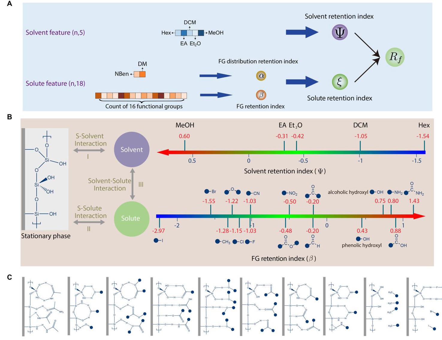
FIGURE 2 | Illustration of the retention indices and their impact on chromatographic behavior. (A) The input features correspond to different retention indices. Here, FG stands for functional group. (B) TLC experiment can be understood as a process where the stationary phase (silica gel) and the mobile phase (solvent) compete for the solute molecules. This competition’s outcome is reflected in the ${R}_{f}$ value. The factors influencing the ${R}_{f}$ value can be categorized into three types: interaction between the stationary phase and the solvent (I), interaction between the stationary phase and the solute (II), and interaction between the solvent and the solute (III). The two retention indices $\left( {\Psi \text{ and }\beta }\right)$ characterize how solvent and solute impact the chromatographic behavior separately. (C) Illustration of interactions between the stationary phase and different functional groups.
图2 | 保留指数及其对色谱行为的影响示意图。(A) 输入特征对应不同的保留指数。这里,FG代表官能团。(B) 薄层色谱实验可以理解为固定相(硅胶)和流动相(溶剂)争夺溶质分子的过程。这种竞争的结果反映在${R}_{f}$值中。影响${R}_{f}$值的因素可分为三类:固定相与溶剂之间的相互作用 (I)、固定相与溶质之间的相互作用 (II) 以及溶剂与溶质之间的相互作用 (III)。两个保留指数$\left( {\Psi \text{ and }\beta }\right)$分别表征溶剂和溶质对色谱行为的影响。(C) 固定相与不同官能团之间的相互作用示意图。
2.1.2 | Retention Indices
2.1.2 | 保留指数
In this study, the stationary phase on the TLC plate is silica gel. The determined ${R}_{f}$ values epitomize a dynamic equilibrium. It reflects the competitive interplay between the highly polar stationary phase and the solute molecules, which are mediated through interactive forces by changing the polarities of the mobile phase during the experiment. This interplay exhibits two primary patterns: the solvent facilitates the upward transit of solute via capillary action; concurrently, solvent molecules intervene by dislodging solute molecules from the stationary phase’s surface, attenuating their interactions (as illustrated in Figure 2). The two retention indices distinctly capture the interaction dynamics between the solvent compound and the silica gel, as well as between the solute molecule and the silica gel. Importantly, our approach enables a quantitative assessment of the aforementioned interactions. In the following paragraphs, we will separately analyze these two indices.
在本研究中,薄层色谱板上的固定相为硅胶。所测定的${R}_{f}$值体现了一种动态平衡。它反映了高极性固定相与溶质分子之间的竞争性相互作用,这种相互作用是通过在实验过程中改变流动相的极性,由相互作用力介导的。这种相互作用呈现出两种主要模式:溶剂通过毛细作用促进溶质向上迁移;同时,溶剂分子通过将溶质分子从固定相表面取代,干预这种相互作用,减弱它们之间的相互作用(如图2所示)。这两种保留指数清晰地捕捉了溶剂化合物与硅胶之间以及溶质分子与硅胶之间的相互作用动态。重要的是,我们的方法能够对上述相互作用进行定量评估。在接下来的段落中,我们将分别分析这两个指数。
2.1.2.1 | Solute Retention Index $\xi$ . Considering that the dataset contains 387 organic compounds, previous research normally involves high-dimensional features (such as MACCS keys with 167 dimensions) and physicochemical descriptors to encode the solute molecule into numerical values. However, the former are often challenging for human understanding, while the latter fails to meet the needs of experimental chemists for rapid polarity evaluation of new compounds. We also conducted a comparison analysis between the solute retention index $\xi$ and several existing physicochemical descriptors, demonstrating the superiority of the solute retention index $\xi$ in the context of TLC experiments.
2.1.2.1 | 溶质保留指数$\xi$ 。考虑到数据集包含387种有机化合物,以往的研究通常涉及高维特征(如167维的MACCS键)和物理化学描述符,以将溶质分子编码为数值。然而,前者往往难以被人类理解,而后者无法满足实验化学家对新化合物快速极性评估的需求。我们还对溶质保留指数$\xi$与几种现有的物理化学描述符进行了比较分析,证明了溶质保留指数$\xi$在薄层色谱实验中的优越性。
To carry out this study, we carefully selected 16 representative functional groups and used their counts as features for the target molecules. Additionally, we characterized the distribution of these functional groups within the molecule by using the number of benzene rings (NBen) and dipole moment (DM). Notably, by further refining the allocation of functional groups within the benzene ring, we were able to improve prediction accuracies; the corresponding results are presented in Supporting Information.
为了开展这项研究,我们精心挑选了16个具有代表性的官能团,并将它们的数量用作目标分子的特征。此外,我们通过苯环数(NBen)和偶极矩(DM)来表征这些官能团在分子内的分布。值得注意的是,通过进一步优化苯环内官能团的分配,我们能够提高预测准确性;相应结果见补充信息。
Although we were able to reduce the feature numbers to 18, establishing an explainable connection between the polarity of the molecule and these input features remain a major challenge.
尽管我们能够将特征数量减少到18个,但在分子极性与这些输入特征之间建立可解释的联系仍然是一个重大挑战。
Therefore, we distinguish between two essential solute characteristics: functional group (FG) counts and their spatial distribution (Figure 2A). Both aspects are critical for elucidating molecular properties, particularly polarity, which profoundly influences molecular behavior in various solvents and reaction environments. FG counts involve 16 predefined structural motifs, offering insights into potential reactivity and solubility. While these counts provide an initial understanding of chemical behavior, molecular properties are not solely additive; linear contributions from groups alone may not fully capture the complexity of chemical phenomena. Thus, the spatial arrangement of these groups is pivotal, as it impacts the molecule’s geometry, interactions, and stereochemical properties, leading to a more comprehensive characterization of molecular polarity. Therefore, we further extracted two indices, namely the FG retention index $\beta$ and the FG distribution retention index $\alpha$ , to isolate these two effects.
因此,我们区分了两种基本的溶质特征:官能团(FG)数量及其空间分布(图2A)。这两个方面对于阐明分子性质,特别是极性至关重要,极性深刻影响分子在各种溶剂和反应环境中的行为。官能团数量涉及16个预定义的结构基序,有助于了解潜在的反应性和溶解性。虽然这些数量提供了对化学行为的初步理解,但分子性质并非仅仅是可加的;仅基团的线性贡献可能无法完全捕捉化学现象的复杂性。因此,这些基团的空间排列至关重要,因为它影响分子的几何形状、相互作用和立体化学性质,从而更全面地表征分子极性。因此,我们进一步提取了两个指数,即FG保留指数$\beta$和FG分布保留指数$\alpha$ ,以分离这两种效应。
Despite the polarity of functional groups being of great interest, there is a lack of quantitative and scalable methods to compare the polarities of different functional groups; in current practice, chemists often rely mainly on qualitative analysis and their experience. Our FG retention index provides the first empirical quantification of the impact of different functional groups on molecular polarity. Considering the 16 functional groups involved in this study, the input features for the sub-model used to obtain the FG retention index $\beta$ consist of ${16}\mathrm{D}$ vectors, with each dimension representing the number of the respective functional group. To quantify the polarity of a specific functional group ${\mathrm{{FG}}}_{i}$ , we configured the input feature vector such that the $i$ -th position was set to 1 and the others to 0 . As illustrated in Figure 2B, the sub-model’s outputs reveal a distinct polarity order among the functional groups, i.e., amides (1.43) > carboxylic acid (0.88) > amine (0.80) > alcoholic hydroxyl (0.75) > phenolic hydroxyl $\left( {0.43}\right) >$ aldehyde $\left( {-{0.20}}\right) >$ ketone $\left( {-{0.20}}\right) >$ ester $\left( {-{0.48}}\right) >$ nitro $\left( {-{0.50}}\right) >$ cyano $\left( {-{1.03}}\right) >$ fluorine $\left( {-{1.03}}\right) >$ chlorine $\left( {-{1.15}}\right) >$ ether (-1.22) > methyl (-1.28) > bromine (-1.55) > iodine (-2.97).
尽管官能团的极性备受关注,但目前缺乏定量且可扩展的方法来比较不同官能团的极性;在当前实践中,化学家通常主要依赖定性分析和经验。我们的官能团保留指数首次对不同官能团对分子极性的影响进行了实证量化。考虑到本研究涉及的16种官能团,用于获得官能团保留指数$\beta$的子模型的输入特征由${16}\mathrm{D}$向量组成,每个维度代表相应官能团的数量。为了量化特定官能团${\mathrm{{FG}}}_{i}$的极性,我们配置输入特征向量,使$i$位置设为1,其他位置设为0。如图2B所示,子模型的输出揭示了官能团之间明显的极性顺序,即酰胺(1.43)>羧酸(0.88)>胺(0.80)>醇羟基(0.75)>酚羟基$\left( {0.43}\right) >$醛$\left( {-{0.20}}\right) >$酮$\left( {-{0.20}}\right) >$酯$\left( {-{0.48}}\right) >$硝基$\left( {-{0.50}}\right) >$氰基$\left( {-{1.03}}\right) >$氟$\left( {-{1.03}}\right) >$氯$\left( {-{1.15}}\right) >$醚(-1.22)>甲基(-1.28)>溴(-1.55)>碘(-2.97)。
To further validate our proposed solute retention index $\xi$ , we conducted a Spearman correlation analysis with established molecular properties. The solute retention index exhibited a moderate positive correlation with $n$ -octanolwater partition coefficient (LogP, ${r}_{s} = {0.50}$ ), indicating that as the LogP values increase, there is a general trend of increasing the solute retention index $\xi$ , suggesting that our index partially captures hydrophobic characteristics. Conversely, the solute retention index $\xi$ showed a moderate negative correlation with topological polar surface area (TPSA, ${r}_{s} = - {0.61}$ ), highlighting that as the TPSA increases, solute retention index $\xi$ tends to decrease, effectively capturing aspects of molecular polarity related to surface area.
为了进一步验证我们提出的溶质保留指数$\xi$,我们与已有的分子性质进行了斯皮尔曼相关性分析。溶质保留指数与$n$-辛醇水分配系数(LogP,${r}_{s} = {0.50}$)呈现中等正相关,这表明随着LogP值增加,溶质保留指数$\xi$总体上有增加的趋势,这意味着我们的指数部分捕捉到了疏水性特征。相反,溶质保留指数$\xi$与拓扑极性表面积(TPSA,${r}_{s} = - {0.61}$)呈现中等负相关,突出表明随着TPSA增加,溶质保留指数$\xi$趋于下降,有效捕捉了与表面积相关的分子极性方面。
For a comprehensive comparison, we employed our solute retention index $\xi$ , MPI, LogP, TPSA, and DM as 1D solute characteristics, using five different solvent volume percentages as 5D solvent characteristics in a model established through the XGBoost model. This analysis is entirely independent of our UHSR model and was conducted to evaluate the predictive capability of $\xi$ in a separate machine learning context. The XGBoost model served as a robust benchmark for evaluating the predictive capability of different solute characteristics.
为了进行全面比较,我们在通过XGBoost模型建立的模型中,将我们的溶质保留指数$\xi$、MPI、LogP、TPSA和DM用作一维溶质特征,将五种不同的溶剂体积百分比用作五维溶剂特征。此分析完全独立于我们的UHSR模型,旨在评估$\xi$在单独的机器学习环境中的预测能力。XGBoost模型作为评估不同溶质特征预测能力的强大基准。
Specifically, we compared the predictive performance of the XGBoost model, as shown in Table 2a. The solute retention index $\xi$ demonstrated superior predictive performance, outperforming other solute descriptors. We also performed tree-based feature importance analyses within the XGBoost model, as detailed in Figure S1. These analyses highlighted the predominant influence of the solute retention index $\xi$ over other traditional descriptors.
具体而言,我们比较了XGBoost模型的预测性能,如表2a所示。溶质保留指数$\xi$表现出卓越的预测性能,优于其他溶质描述符。我们还在XGBoost模型中进行了基于树的特征重要性分析,如图S1详细所示。这些分析突出了溶质保留指数$\xi$相对于其他传统描述符的主要影响。
2.1.2.2 | Solvent Retention Index Ψ. Chromatographic retention on silica gel results from the synergistic interplay of electrostatic (dipole-dipole and ion-dipole), hydrogen-bonding, and van der Waals dispersion forces; molecular polarity alone represents only one component of this adsorption mechanism. Accordingly, we define the solvent retention index $\Psi$ as an empirical measure of the net adsorption strength of each pure solvent on silica.
2.1.2.2 | 溶剂保留指数Ψ。硅胶上的色谱保留是由静电(偶极-偶极和离子-偶极)、氢键和范德华色散力的协同相互作用产生的;仅分子极性只是这种吸附机制的一个组成部分。因此,我们将溶剂保留指数$\Psi$定义为每种纯溶剂在硅胶上净吸附强度的实证度量。
Methanol (MeOH), with one hydrogen-bond donor (HBD) and one acceptor (HBA), forms both six- and eight-membered chelates with the surface silanol and siloxane groups (see Figure 2C). Ethyl acetate (EA) features two HBAs that engage in an eight-membered ring complex via its ester oxygens. Diethyl ether $\left( {{\mathrm{{Et}}}_{2}\mathrm{O}}\right)$ has a single HBA, allowing only one hydrogen-bonding mode. Dichloromethane (DCM), bearing two chlorides, interacts primarily through weaker dipole-dipole and dispersion forces. In contrast, $n$ -hexane (Hex) adsorbs only via weak dispersion interactions and cannot displace more strongly adsorbing solvents. Under this framework, the adsorption hierarchy is
甲醇(MeOH)有一个氢键供体(HBD)和一个受体(HBA),它与表面硅醇和硅氧烷基团形成六元环和八元环螯合物(见图2C)。乙酸乙酯(EA)有两个HBA,通过其酯氧形成八元环络合物。二乙醚$\left( {{\mathrm{{Et}}}_{2}\mathrm{O}}\right)$有一个单一的HBA,只允许一种氢键模式。二氯甲烷(DCM)有两个氯原子,主要通过较弱的偶极 - 偶极和色散力相互作用。相比之下,$n$ -己烷(Hex)仅通过弱色散相互作用吸附,无法取代吸附更强的溶剂。在此框架下,吸附层次结构为
$$ \mathrm{{MeOH}} > \mathrm{{EA}} > {\mathrm{{Et}}}_{2}\mathrm{O} > \mathrm{{DCM}} > \mathrm{{Hex}}\text{ . } $$The input features of the sub-model used to obtain $\Psi$ consist of 5D vectors, with each dimension representing the volume percentage of a solvent compound. Consequently, variations in the compound ratio within the solvent system directly influence the value of $\Psi$ , thereby changing the polarity of the solvent. Moreover, to isolate the effect of each compound, we can assign the value 1 to the volume percentage that corresponds to the target solvent compound, while setting the others to 0 . This approach yields the following values (see Figure 2B):
用于获得$\Psi$的子模型的输入特征由5D向量组成,每个维度代表一种溶剂化合物的体积百分比。因此,溶剂系统中化合物比例的变化直接影响$\Psi$的值,从而改变溶剂的极性。此外,为了分离每种化合物的影响,我们可以将与目标溶剂化合物对应的体积百分比赋值为1,而将其他值设为0。这种方法得出以下值(见图2B):
$$ {\Psi }_{\mathrm{{Hex}}} = - {1.54},{\Psi }_{\mathrm{{DCM}}} = - {1.05},{\Psi }_{{\mathrm{{Et}}}_{2}\mathrm{O}} = - {0.42}, $$$$ {\Psi }_{\mathrm{{EA}}} = - {0.31},{\Psi }_{\mathrm{{MeOH}}} = {0.60} $$Comparison with experimental miscibility indices (LogP and aqueous solubility [43]) confirms that $\Psi$ captures the combined electrostatic, hydrogen-bonding, and dispersion contributions to solvent-silica adsorption (see Table 2b).
与实验混溶指数(LogP和水溶性[43])的比较证实,$\Psi$捕捉了对溶剂 - 二氧化硅吸附的静电、氢键和色散综合贡献(见表2b)。
TABLE 2 | Comparison of (a) solute retention index $\xi$ and (b) solvent retention index $\Psi$ with established physicochemical descriptors.
表2 | (a)溶质保留指数$\xi$和(b)溶剂保留指数$\Psi$与已建立的物理化学描述符的比较。
| (a) Comparison of model performance of solute retention index $\xi$ with other established physicochemical descriptors | ||||
| Solute feature (with fixed 5 solvent features) | ${\mathbf{R}}^{2}$ | RMSE | ${r}_{s}$ (with ${R}_{f}$ value) | ${r}_{s}$ (with solute retention index $\xi$ ) |
| Solute retention index $\xi$ | 0.95 | 0.070 | 0.63 | - |
| LogP | 0.79 | 0.15 | 0.33 | 0.50 |
| MPI | 0.81 | 0.14 | -0.23 | -0.34 |
| Dipole Moment | 0.73 | 0.18 | -0.06 | -0.08 |
| TPSA | 0.81 | 0.15 | -0.40 | -0.61 |
(b) Comparison of solvent retention index $\Psi$ with estabilished solvent properties
(b)溶剂保留指数$\Psi$与已确定的溶剂性质的比较
| Solubility in water | |||||
| Solvent | HBD | HBA | (g/100g) [43] | LogP | $\Psi$ |
| Hex | 0 | 0 | 0.01 | 3.42 | -1.54 |
| DCM | 0 | 0 | 1.32 | 1.01 | -1.05 |
| ${\mathrm{{Et}}}_{2}\mathrm{O}$ | 0 | 1 | 6.9 | 0.76 | -0.42 |
| EA | 0 | 2 | 7.7 | 0.29 | -0.31 |
| MeOH | 1 | 1 | Miscible | -0.27 | 0.60 |
2.2 | The ${R}_{f}$ Governing Equation
2.2 | ${R}_{f}$的控制方程
To comprehensively understand the relationship between the ${R}_{f}$ value and the two retention indices, we used symbolic regression to formulate empirical mathematical expressions connecting the ${R}_{f}$ value and the two retention indices (Figure 3A). The observed ${R}_{f}$ values were obtained directly from our automatic high-throughput platform [17], while the computed ${R}_{f}$ values were calculated from the ${R}_{f}$ governing equation (see Equation 1 below).
为了全面理解${R}_{f}$值与两个保留指数之间的关系,我们使用符号回归来构建连接${R}_{f}$值与两个保留指数的经验数学表达式(图3A)。观测到的${R}_{f}$值直接来自我们的自动高通量平台[17],而计算得到的${R}_{f}$值则根据${R}_{f}$控制方程计算得出(见下面的方程1)。
To ensure that the computed ${R}_{f}$ values lie within the range from 0 to 1, a sigmoidal function was employed (see Figure 3B). By using symbolic regression, one obtains several candidates for the ${R}_{f}$ governing equation (see Table S1). Since a simple formula is desired, and considering the prescribed fitting accuracy $\left( {{R}^{2} = }\right. \; {0.908},\mathrm{{RMSE}} = {0.104})$ , we selected
为确保计算得到的${R}_{f}$值在0到1的范围内,采用了一个S形函数(见图3B)。通过使用符号回归,可以得到几个${R}_{f}$控制方程的候选式(见表S1)。由于需要一个简单的公式,并考虑规定的拟合精度$\left( {{R}^{2} = }\right. \; {0.908},\mathrm{{RMSE}} = {0.104})$,我们选择了……
$$ {R}_{f} = \sigma \left( {{5.15\Psi } + {5.15\xi } + {1.55}}\right) ,\;\sigma \left( x\right) = \frac{1}{1 + {e}^{-x}}. \tag{1} $$In order to separately analyze the individual influence of solvent and solute on the ${R}_{f}$ value, we further decomposed the formula for ${R}_{f}$ in Equation 1 into $h\left( \Psi \right)$ and $g\left( \xi \right)$ . For instance, as illustrated in Figure 3C, when considering a specific solute molecule (i.e., fixing a value for the solute retention index $\xi$ ), we can reformulate Equation 1 as ${R}_{f} = h\left( \Psi \right) = \sigma \left( {{5.15\Psi } + {C}_{1}}\right)$ , where ${C}_{1}$ depends on the chosen solute molecule. The pattern observed in Figure 3C shows that ${R}_{f}$ increases with the solvent retention index $\Psi$ . Since a larger value of solvent retention index $\Psi$ indicates greater polarity, this finding emphasizes that the solvent retention index $\Psi$ correlates with the polarity of the solvent. Furthermore, we observe that the shape of $h\left( \Psi \right)$ ’s graph varies significantly for different solute molecules. In particular, Figure 3C indicates that, within the context of our dataset, changing the solvent’s composition only has a subtle effect on ${R}_{f}$ for solute molecules with extreme polarities. Similarly, when the solvent is fixed, Equation 1 can be reformulated as ${R}_{f} = g\left( \xi \right) = \sigma \left( {{5.15\xi } + {C}_{2}}\right)$ , where ${C}_{2}$ depends on the chosen value for the solvent retention index $\Psi$ . By analysis similar to the previous case (fixed solute), the ${R}_{f}$ value increases with the solute retention index $\xi$ . But now, a larger value of the solute retention index $\xi$ indicates a lower polarity. Moreover, we observe that the shape of $g\left( \xi \right)$ ’s graph is of the same $S$ -shaped type across different solvent systems (see Figure 3C).
为了分别分析溶剂和溶质对${R}_{f}$值的单独影响,我们进一步将方程1中${R}_{f}$的公式分解为$h\left( \Psi \right)$和$g\left( \xi \right)$。例如,如图3C所示,当考虑一个特定的溶质分子(即固定溶质保留指数$\xi$的值)时,我们可以将方程1重新表述为${R}_{f} = h\left( \Psi \right) = \sigma \left( {{5.15\Psi } + {C}_{1}}\right)$,其中${C}_{1}$取决于所选的溶质分子。图3C中观察到的模式表明,${R}_{f}$随着溶剂保留指数$\Psi$的增加而增加。由于溶剂保留指数$\Psi$的值越大表明极性越大,这一发现强调了溶剂保留指数$\Psi$与溶剂的极性相关。此外,我们观察到$h\left( \Psi \right)$的图形形状因不同的溶质分子而有显著变化。特别是,图3C表明,在我们的数据集中,对于具有极端极性的溶质分子,改变溶剂的组成对${R}_{f}$只有微妙的影响。同样,当溶剂固定时,方程1可以重新表述为${R}_{f} = g\left( \xi \right) = \sigma \left( {{5.15\xi } + {C}_{2}}\right)$,其中${C}_{2}$取决于所选的溶剂保留指数$\Psi$的值。通过与前面情况(固定溶质)类似的分析,${R}_{f}$值随着溶质保留指数$\xi$的增加而增加。但现在,溶质保留指数$\xi$的值越大表明极性越低。此外,可以观察到,在不同的溶剂系统中,$g\left( \xi \right)$的图形形状是相同的$S$形(见图3C)。
Due to the limitations of the data, different modular neural networks can achieve similar accuracy. However, we observed that while the retention indices change, the discovered ${R}_{f}$ equations maintain a similar form with varying parameters, as illustrated in Tables S10-S12. In TLC experiments, the absolute values of the retention indices are less crucial than their relative values. The relative values of the retention indices are what guide the separation process in TLC. Given that the underlying equations maintain a similar form, variations in the retention indices can be viewed as differences in units rather than changes in fundamental properties. For example, given a target molecule and two solvent systems (e.g., the polarity of the first solvent system is smaller than the second solvent system), we may obtain two sets of solvent retention indices $\left( {{\Psi }_{1},{\Psi }_{2}}\right)$ and $\left( {{\Psi }_{1}^{\prime },{\Psi }_{2}^{\prime }}\right)$ , the relative relationship maintain the same, i.e., ${\Psi }_{1} < {\Psi }_{2},{\Psi }_{1}^{\prime } < {\Psi }_{2}^{\prime }$ .
由于数据的局限性,不同的模块化神经网络可以达到相似的精度。然而,我们观察到,虽然保留指数发生了变化,但发现的${R}_{f}$方程在参数变化时保持相似的形式,如表S10 - S12所示列。在薄层色谱实验中,保留指数的绝对值不如其相对值重要。保留指数的相对值指导着薄层色谱中的分离过程。鉴于基本方程保持相似的形式,保留指数的变化可以看作是单位上的差异,而不是基本性质的变化。例如,对于一个目标分子和两种溶剂系统(例如,第一种溶剂系统的极性小于第二种溶剂系统),我们可能会得到两组溶剂保留指数$\left( {{\Psi }_{1},{\Psi }_{2}}\right)$和$\left( {{\Psi }_{1}^{\prime },{\Psi }_{2}^{\prime }}\right)$,它们的相对关系保持不变,即${\Psi }_{1} < {\Psi }_{2},{\Psi }_{1}^{\prime } < {\Psi }_{2}^{\prime }$。
2.3 | Quantification of Solvent Polarity
2.3 | 溶剂极性的量化
In addition to characterizing the polarity of the eluent solvent, the UHSR framework offers an explainable solution for understanding how different compounds influence the solvent retention index $\Psi$ . In this study, we consider five distinct solvent compounds: Hex, EA, DCM, MeOH, and ${\mathrm{{Et}}}_{2}\mathrm{O}$ . To achieve the designed solvent polarity, chemists usually adjust the ratios of these compounds in the mobile phase system. By directly applying the SR algorithm, we obtained the empirical mathematical equation between solvent retention index $\Psi$ and its corresponding input variables, i.e., the volume ratio of $\mathrm{{Hex}},\mathrm{{DCM}},{\mathrm{{Et}}}_{2}\mathrm{O},\mathrm{{EA}}$ , and $\mathrm{{MeOH}}$ in the mobile phase system. The following formula achieved a high ${R}^{2}$ of 0.956 and a low RMSE of 0.069 with a simple form,
除了表征洗脱剂溶剂的极性外,UHSR框架还为理解不同化合物如何影响溶剂保留指数$\Psi$提供了一种可解释的解决方案。在本研究中,我们考虑了五种不同的溶剂化合物:己烷、乙酸乙酯、二氯甲烷、甲醇和${\mathrm{{Et}}}_{2}\mathrm{O}$。为了实现设计的溶剂极性,化学家通常会调整这些化合物在流动相系统中的比例。通过直接应用SR算法,我们获得了溶剂保留指数$\Psi$与其相应输入变量之间的经验数学方程,即流动相系统中$\mathrm{{Hex}},\mathrm{{DCM}},{\mathrm{{Et}}}_{2}\mathrm{O},\mathrm{{EA}}$、$\mathrm{{MeOH}}$的体积比。以下公式以简单的形式实现了0.956的高${R}^{2}$和0.069的低均方根误差。
$$ \Psi = - {1.37}\mathrm{{Hex}} - {0.20}\mathrm{{EA}} - {1.02}\mathrm{{DCM}} + {4.65}\mathrm{{MeOH}} - {0.45}{\mathrm{{Et}}}_{2}\mathrm{O}\text{ . } $$(2)
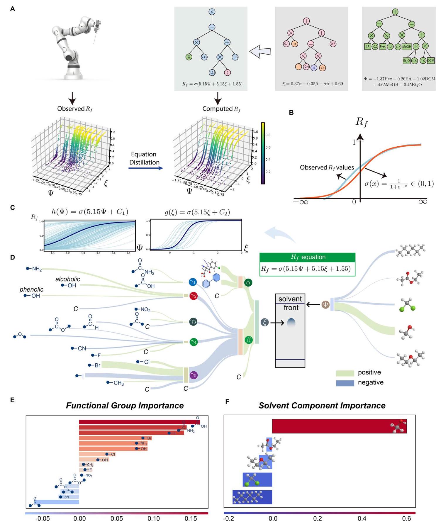
FIGURE 3 | Visualization of the latent variables and the decomposition of the retrieved formula. (A) Visualization of the observed and calculated ${R}_{f}$ values with two retention indices solvent retention index $\Psi$ and solute retention index $\xi$ . (B) Fitting observed ${R}_{f}$ values with a Sigmoid function. (C) Decomposition of Equation 1 into $h\left( \Psi \right)$ and $g\left( \xi \right)$ . (D) Visualization the flow of how input variables contribute to the ${R}_{f}$ value, here $C$ represents a constant. (E) Importance of functional groups in determining the functional group retention index ( $\beta$ ). (F) Importance of solvent components in determining the solvent retention index $\left( \Psi \right)$ .
图3 | 潜在变量的可视化和检索公式的分解。(A) 用两个保留指数(溶剂保留指数$\Psi$和溶质保留指数$\xi$)对观察到的和计算出的${R}_{f}$值进行可视化。(B) 用Sigmoid函数拟合观察到的${R}_{f}$值。(C) 将方程1分解为$h\left( \Psi \right)$和$g\left( \xi \right)$。(D) 可视化输入变量如何对${R}_{f}$值产生贡献的流程,这里$C$代表一个常数。(E) 官能团在确定官能团保留指数($\beta$)中的重要性。(F) 溶剂成分在确定溶剂保留指数$\left( \Psi \right)$中的重要性。
Specifically, there are three mobile phase systems involved in the dataset, which are Hex/EA, Hex/Et, O, and MeOH/DCM. Equation 2 quantifies the impact of the two compounds on solvent polarity within each system. For instance, in the presence of Hex and EA, the solvent retention index $\Psi$ is calculated as $\Psi = - {1.37}\mathrm{{Hex}} - {0.20}\mathrm{{EA}}$ . As the volume of EA increases and the volume of Hex decreases, the solvent polarity exhibits a corresponding increase. Moreover, the constant term of 4.65 with MeOH indicates that even a slight increase/decrease in the volume of MeOH will lead to a significant increase/decrease in solvent polarity.
具体来说,数据集中涉及三个流动相系统,分别是己烷/乙酸乙酯、己烷/乙醚、O和甲醇/二氯甲烷。方程2量化了每个系统中两种化合物对溶剂极性的影响。例如,在存在己烷和乙酸乙酯的情况下,溶剂保留指数$\Psi$计算为$\Psi = - {1.37}\mathrm{{Hex}} - {0.20}\mathrm{{EA}}$。随着乙酸乙酯体积的增加和己烷体积的减少,溶剂极性相应增加。此外,甲醇的常数项4.65表明,即使甲醇体积有轻微的增加/减少,也会导致溶剂极性有显著的增加/减少。
2.4 | Quantification of Solute Polarity
2.4 | 溶质极性的量化
As discussed earlier, we introduce two additional functional group-related indices, FG distribution retention index $\alpha$ and FG retention index $\beta$ , to enhance our understanding of the relationship between the molecular polarity and the molecular structure. With the help of symbolic regression, we obtained an explicit mathematical relationship between $\xi$ and $\left( {\alpha ,\beta }\right)$ as follows:
如前所述,我们引入了另外两个与官能团相关的指数,FG分布保留指数$\alpha$和FG保留指数$\beta$,以加深我们对分子极性与分子结构之间关系的理解。借助符号回归,我们得到了$\xi$和$\left( {\alpha ,\beta }\right)$之间的明确数学关系如下:
$$ \xi = {0.37\alpha } - {0.35\beta } - {\alpha \beta } + {0.69}. \tag{3} $$Breaking down Equation 3, the molecular polarity can be understood as a combination of the effect of functional groups’ distribution $\left( {{f}_{1}\left( \alpha \right) = {0.37\alpha }}\right)$ , the contribution of the functional groups within the molecule $\left( {{f}_{2}\left( \beta \right) = - {0.35\beta }}\right)$ and the interaction between these two factors $\left( {{f}_{3}\left( {\alpha ,\beta }\right) = - {\alpha \beta }}\right)$ .
分解方程3,分子极性可以理解为官能团分布$\left( {{f}_{1}\left( \alpha \right) = {0.37\alpha }}\right)$的影响、分子内官能团的贡献$\left( {{f}_{2}\left( \beta \right) = - {0.35\beta }}\right)$以及这两个因素之间的相互作用$\left( {{f}_{3}\left( {\alpha ,\beta }\right) = - {\alpha \beta }}\right)$的组合。
To perform a finer-grain analysis of the individual impacts of $\alpha$ and $\beta$ on molecular polarity, we further derived specific equations that decompose the contributions of each feature, as follows,
为了对$\alpha$和$\beta$对分子极性的个体影响进行更细粒度的分析,我们进一步推导了分解每个特征贡献的具体方程,如下所示,
$$ \alpha = \left( {\mathrm{{DM}} + \mathrm{{NBen}} - {0.29}}\right) \left( {-\mathrm{{NBen}} \cdot {e}^{\mathrm{{DM}} - \mathrm{{NBen}}} + {2.28} \cdot {e}^{\mathrm{{DM}} - \mathrm{{NBen}}}}\right. $$$$
- {0.64}\mathrm{{NBen}} + {1.66}) - {0.74}\text{ , } \tag{4a} $$
where
其中
$$ \begin{cases} {\gamma }_{1} = & {5.16C}{\mathrm{t}}_{\mathrm{{Am}}} + {5.16}\log \left( {C{\mathrm{t}}_{{\mathrm{C}}_{12}\mathrm{H}} + {0.86}}\right) , \\ {\gamma }_{2} = & {3.83C}{\mathrm{t}}_{\mathrm{{Ph}}} + {8.70}\left( {C{\mathrm{t}}_{{\mathrm{{RBH}}}_{2}} + C{\mathrm{t}}_{\mathrm{{OH}}}}\right) - {0.73}, \\ {\gamma }_{3} = & \frac{C{\mathrm{t}}_{{\mathrm{{NO}}}_{2}} + C{\mathrm{t}}_{{\mathrm{{RCO}}}_{2}\mathrm{R}}}{\Delta + 1} - {0.29}, \\ {\gamma }_{4} = & C{\mathrm{t}}_{{\mathrm{{RC}}}_{2}} + C{\mathrm{t}}_{{\mathrm{{RC}}}_{12}\mathrm{R}} + {1.44}) - {2.96C}{\mathrm{t}}_{{\mathrm{R}}_{2}\mathrm{C}\mathrm{e} - 2} - {2.96}{e}^{C{\mathrm{t}}_{{\mathrm{R}}_{2}}} \\ & - {2.96}\left( {C{\mathrm{t}}_{\mathrm{L}} + {0.66}}\right) ,\left( {C{\mathrm{t}}_{{\mathrm{{RC}}}_{2}\mathrm{C}\mathrm{e} + C} + C{\mathrm{t}}_{\mathrm{{RC}}\mathrm{B}} + C{\mathrm{t}}_{\mathrm{C}\mathrm{N}} - {1.20}}\right) , \\ {\gamma }_{5} = & C{\mathrm{t}}_{{\mathrm{{RC}}}_{2}} + {2.54C}{\mathrm{t}}_{\mathrm{C}} + {2.54}\left( {{1.21} - C{\mathrm{t}}_{\mathrm{R}}}\right) \\ & - {1.30}, \\ & - {1.30}, \end{cases} $$(5)
The above equations are indeed more complex and less directly interpretable than the top-level ${R}_{f}$ equation (Equation 1). This complexity arises from the intricate nature of molecular polarity, which involves nonlinear interactions between functional groups and structural features. While the top-level ${R}_{f}$ equation is designed to provide a concise, human-readable relationship between solute polarity, solvent polarity, and the ${R}_{f}$ value, serving as a conceptual tool for understanding how polarity indices influence ${R}_{f}$ values, the more detailed Equations (4) and (5) serve a different purpose. These equations function as computational tools to calculate latent chemical properties, such as $\alpha$ and $\beta$ , from molecular structures. By incorporating terms like ${\gamma }_{1}$ to ${\gamma }_{5}$ , they enable precise quantification of the contributions of specific functional groups and their interactions, which would otherwise be difficult to disentangle.
上述方程确实比顶级${R}_{f}$方程(方程1)更复杂且不太直接可解释。这种复杂性源于分子极性的复杂性质,它涉及官能团和结构特征之间的非线性相互作用。虽然顶级${R}_{f}$方程旨在提供溶质极性、溶剂极性和${R}_{f}$值之间简洁、易于理解的关系,作为理解极性指数如何影响${R}_{f}$值的概念工具,但更详细的方程(4)和(5)有不同的用途。这些方程用作计算工具,从分子结构计算潜在的化学性质,如$\alpha$和$\beta$。通过纳入${\gamma }_{1}$到${\gamma }_{5}$等项,它们能够精确量化特定官能团的贡献及其相互作用,否则这些贡献将难以区分。
Although these detailed equations are not intended for direct human interpretation, their value lies in supporting downstream analyses, such as feature importance assessments and visualizations. These analyses, introduced in the following subsection, help bridge the gap between computational complexity and practical insights, making the results more accessible and actionable for researchers.
虽然这些详细方程并非用于直接的人工解释,但其价值在于支持下游分析,如特征重要性评估和可视化。在下一小节中介绍的这些分析有助于弥合计算复杂性与实际见解之间的差距,使结果对研究人员更易于理解和操作。
2.5 | Visualization of the Discovered Equations
2.5 | 发现方程的可视化
To understand how the discovered equations explain the relationship between input features and the final ${R}_{f}$ value prediction, we utilized two complementary visualization approaches: feature importance visualization and direct value contribution visualization. These methods provide different but synergistic perspectives on how features influence the final ${R}_{f}$ values.
为了理解发现的方程如何解释输入特征与最终${R}_{f}$值预测之间的关系,我们采用了两种互补的可视化方法:特征重要性可视化和直接值贡献可视化。这些方法从不同但协同的角度展示了特征如何影响最终的${R}_{f}$值。
Feature importance quantifies the sensitivity of the model output to variations in individual input features. Through the derived equations, we can directly identify which features have the most significant impact on the ${R}_{f}$ prediction. For example, as shown in Figure 3E, the count of halogen atoms (e.g., iodine) and the carboxylic acid group $\left( {\mathrm{{Ct}}}_{{\mathrm{{CO}}}_{2}\mathrm{H}}\right)$ are identified as features with high importance. As shown in Figure 3F, methanol (MeOH) plays a significant role in influencing the ${R}_{f}$ values. This approach is particularly useful for identifying the key drivers of variability in the model’s predictions across the dataset. In addition to understanding feature importance, we also visualized the direct numerical contribution of each input variable to a specific prediction. This approach traces how the “value” of each feature propagates through the discovered equations to influence the final ${R}_{f}$ value. As shown in Figure 3D, this step-by-step visualization reveals how input variables contribute to intermediate indices (e.g., ${\gamma }_{1},\beta ,\xi$ ) and ultimately to ${R}_{f}$ .
特征重要性量化了模型输出对各个输入特征变化的敏感性。通过推导的方程,我们可以直接确定哪些特征对${R}_{f}$预测有最显著的影响。例如,如图3E所示,卤原子(如碘)的数量和羧酸基团$\left( {\mathrm{{Ct}}}_{{\mathrm{{CO}}}_{2}\mathrm{H}}\right)$被确定为具有高重要性的特征。如图3F所示,甲醇(MeOH)在影响${R}_{f}$值方面起着重要作用。这种方法对于识别整个数据集中模型预测变化的关键驱动因素特别有用。除了理解特征重要性,我们还可视化了每个输入变量对特定预测的直接数值贡献。这种方法追踪每个特征的“值”如何通过发现的方程传播以影响最终的{{F}}值。如图3D所示,这种逐步可视化揭示了输入变量如何对中间指标(如${\gamma }_{1},\beta ,\xi$)做出贡献并最终影响${R}_{f}$。
For instance, if the count of iodine is set to 1 , we can directly observe how this value influences ${\gamma }_{5}$ , which then propagates to $\beta$ , and finally contributes to the ${R}_{f}$ value. Unlike feature importance, which focuses on sensitivity to changes, this approach provides a numerical breakdown of how much each input feature contributes to the final prediction for a given input configuration.
例如,如果碘的数量设置为1,我们可以直接观察到这个值如何影响${\gamma }_{5}$,然后传播到$\beta$,最终对${R}_{f}$值做出贡献。与关注变化敏感性的特征重要性不同,这种方法提供了每个输入特征对给定输入配置的最终预测贡献多少的数值分解。
While feature importance highlights which features are most critical across the dataset, direct value contribution visualization, provides a more detailed view of how the equations process specific inputs. Together, these visualizations offer a comprehensive understanding of the discovered equations, allowing us to both identify key features and trace their influence on the ${R}_{f}$ value.
虽然特征重要性突出了数据集中哪些特征最关键,但直接值贡献可视化提供了方程如何处理特定输入的更详细视图。这些可视化方法一起提供了对发现方程的全面理解,使我们既能识别关键特征,又能追踪它们对${R}_{f}$值的影响。
2.6 | Chemists’ Evaluation on UHSR
2.6 | 化学家对UHSR的评估
2.6.1 | Survey Evaluation
2.6.1 | 调查评估
To thoroughly assess whether the UHSR model thinks like chemists, we grounded our evaluation using the judgments of chemists. We conducted a comprehensive survey involving 100 chemists with an average of 10 years of experience in the field of chemistry. Please see the complete survey in the Supporting Information.
为了全面评估UHSR模型的思维方式是否与化学家一致,我们以化学家的判断为基础进行评估。我们对100位平均拥有10年化学领域经验的化学家进行了全面调查。完整的调查内容请见补充信息。
According to the survey results, an impressive 97.0% of the chemists indicated that the retention indices derived from the UHSR model align well with their expectations based on their professional experience (see Figure 4A). This high level of alignment shows the model’s ability to capture key aspects of molecular polarity that are consistent with established chemical principles. Similarly, 99.0% of the chemists agreed that the ${R}_{f}$ governing equation meets their expectations. This suggests that the model’s predictions are not only accurate but also resonate with the intuitive understanding of chemists. 99.0% of the respondents felt that the retention indices and the governing equation provided new insights and knowledge. These results indicate that the qualitative concepts chemists had accumulated over time align with the quantitative equations we discovered. Our quantitative equations provide a structured and solidified description of the intuitive conclusions that chemists have developed through their experiences. This solidification of qualitative concepts into quantitative forms offers a valuable bridge between empirical knowledge and rigorous scientific modeling.
根据调查结果,令人印象深刻的是,97.0%的化学家表示,基于他们的专业经验,UHSR模型得出的保留指数与他们的预期高度吻合(见图4A)。这种高度的吻合表明该模型能够捕捉与既定化学原理一致的分子极性的关键方面。同样,99.0%的化学家认为${R}_{f}$控制方程符合他们的预期。这表明该模型的预测不仅准确,而且与化学家的直观理解相呼应。99.0%的受访者认为保留指数和控制方程提供了新的见解和知识。这些结果表明,化学家们长期积累的定性概念与我们发现的定量方程是一致的。我们的定量方程为化学家们通过经验得出的直观结论提供了结构化和固化的描述。这种将定性概念固化为定量形式的做法在经验知识和严谨的科学建模之间架起了一座宝贵的桥梁。
To better understand chemists’ preference between the UHSR model and traditional machine learning models (such as artificial neural networks), we categorized the chemists into three levels based on their levels of expertise in AI knowledge [44]: Level 1 indicates minimal AI knowledge, Level 2 indicates moderate AI knowledge, and Level 3 indicates extensive AI knowledge. As shown in Figure 4A, among chemists with Level 3 AI knowledge, 88.2% of chemists expressed a higher level of trust in the UHSR model compared to traditional machine learning models, and the remaining showed no preference between the two types of models. Among chemists with Level 2 AI knowledge, 44.6% trusted the UHSR model more, 43.1% had no preference, and only 12.3% trusted the black box model more. For chemists with minimal AI knowledge, 55.6% of the chemists showed no preference, while 22.2% trusted the UHSR model more. This finding suggests that the transparency and interpretability of the UHSR model are particularly appreciated by those with a deeper understanding of AI.
为了更好地了解化学家在UHSR模型和传统机器学习模型(如人工神经网络)之间的偏好,我们根据他们在人工智能知识方面的专业水平将化学家分为三个级别[44]:1级表示人工智能知识最少,2级表示中等人工智能知识,3级表示广泛的人工智能知识。如图4A所示,在拥有3级人工智能知识的化学家中,88.2%的化学家对UHSR模型的信任度高于传统机器学习模型,其余的人对这两种模型没有偏好。在拥有2级人工智能知识的化学家中,44.6%的人更信任UHSR模型,43.1%的人没有偏好,只有12.3%的人更信任黑箱模型。对于人工智能知识最少的化学家来说,55.6%的化学家没有偏好,而22.2%的人更信任UHSR模型。这一发现表明,UHSR模型的透明度和可解释性尤其受到对人工智能有更深入理解的人的赞赏。
2.6.2 | Experimental Evaluation
2.6.2 | 实验评估
Furthermore, it is crucial to recommend solvent ratios for column chromatography by examining the positioning of compounds in TLC experiments under various solvent ratios. Ideally, the solvent ratio should maximize the difference in ${R}_{f}$ values between the components to be separated, or place the target molecule’s ${R}_{f}$ value between 0.2 and 0.3 [45]. Based on this approach, we explored the consistency of the optimal solvent ratio between the UHSR model (an AI model trained from standardized data) and experimental data under non-standardized experimental conditions (such as different TLC plates, temperature, humidity, and time). Here, we examined the product o-hydroxybenzaldehyde 2 and $p$ -hydroxybenzaldehyde 3 of the Reimer-Tiemann reaction [46] from phenol 1 were detected by thin-layer chromatography (Figure 4B). At different solvent ratios, there was a high correlation between ${R}_{f}$ values of the manual TLC experiment (Exp.) and predicted values of UHSR. By analyzing the ${R}_{f}$ differences between component pairs across 19 different solvent ratios for five solvents, we found that 7 out of 9 optimal solvent ratios recommended by UHSR predictions matched the experimental data, demonstrating the robustness of our model under a variety of experimental conditions. Additionally, the quantification of solvent polarity for the recommended optimal solvent ratios was determined using the proposed solvent retention index $\Psi$ . It was observed that some of these optimal solvent ratios exhibit similar polarity.
此外,通过在各种溶剂比例下的薄层色谱实验中检查化合物的位置来推荐柱色谱的溶剂比例至关重要。理想情况下,溶剂比例应使待分离组分之间的${R}_{f}$值差异最大化,或将目标分子的${R}_{f}$值置于0.2至0.3之间[45]。基于此方法,我们探索了UHSR模型(一个从标准化数据训练的人工智能模型)推荐的最佳溶剂比例与非标准化实验条件下(如不同的薄层板、温度、湿度和时间)的实验数据之间的一致性。在此,我们通过薄层色谱法检测了苯酚1经瑞穆尔-悌曼反应生成的产物邻羟基苯甲醛2和$p$-羟基苯甲醛3(图4B)。在不同的溶剂比例下,手动薄层色谱实验(Exp.)的${R}_{f}$值与UHSR的预测值之间存在高度相关性。通过分析五种溶剂在19种不同溶剂比例下组分对之间的${R}_{f}$差异,我们发现UHSR预测推荐的9种最佳溶剂比例中有7种与实验数据匹配,这表明我们的模型在各种实验条件下具有稳健性。此外,使用提出的溶剂保留指数$\Psi$确定了推荐的最佳溶剂比例的溶剂极性量化。观察到其中一些最佳溶剂比例表现出相似的极性。
2.7 | Transferability and Broader Applications of the UHSR Framework
2.7 | UHSR框架的可转移性和更广泛应用
2.7.1 | Extension to Column Chromatography
2.7.1 | 柱色谱法的扩展
Column chromatography (CC) can be viewed as a natural preparative-scale extension of the structure-polarity principles that govern TLC behavior. To evaluate the effectiveness of our UHSR framework in CC, we employ the same chemically interpretable molecular features listed in Table 1 (e.g. functional group counts) alongside solvent composition parameters (volume percentages of mobile phase components), utilizing experimental data from an automated CC platform [47].
柱色谱法(CC)可被视为支配薄层色谱行为的结构 - 极性原理在制备规模上的自然扩展。为了评估我们的UHSR框架在柱色谱法中的有效性,我们采用了表1中列出的相同的具有化学可解释性的分子特征(例如官能团计数)以及溶剂组成参数(流动相成分的体积百分比),利用来自自动化柱色谱平台的实验数据[47]。
In CC optimization, two critical volume metrics are defined: ${v}_{1}$ , the eluent volume consumed when the target compound begins eluting (corresponding to retention factor $k$ ), and ${v}_{2}$ , the total eluent volume required for complete compound elution (incorporating peak broadening effects). These volumes are predicted through polarity-governing equations:
在柱色谱法优化中,定义了两个关键体积指标:${v}_{1}$,即目标化合物开始洗脱时消耗的洗脱剂体积(对应保留因子$k$),以及${v}_{2}$,即化合物完全洗脱所需的总洗脱剂体积(包括峰展宽效应)。这些体积通过极性控制方程进行预测:
$$ {v}_{1} = {0.25\theta }{\left( \frac{\theta }{\mu }\right) }^{3} - {0.27\theta }\frac{\theta }{\mu } + {0.27\theta } + {6.50}, $$$$ {v}_{2} = {0.006}{\left( \frac{\theta \left( {\theta + \mu }\right) }{\mu - 1} - {13.9}\right) }^{2} + {0.003}{\left( \theta + {0.86}\mu + {1.72}\right) }^{2} $$$$
- {1.94}\frac{\mu }{\theta } - {25.5}\frac{1}{\theta } + {25.1} $$
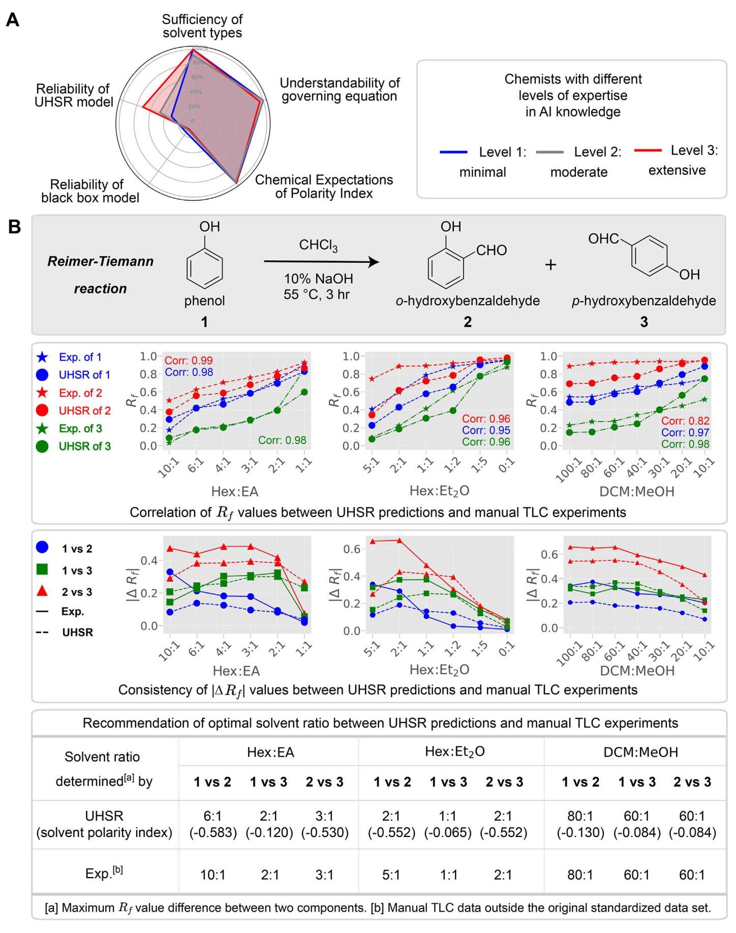
FIGURE 4 | Analysis of the survey and model-experimental data correlation. (A) Survey analysis from chemists with varying levels of AI expertise. (B) Assessment of the consistency between the UHSR model (AI model trained on standardized data) and manual experimental (Exp.) data (nonstandardized experimental conditions, such as different TLC plates, temperatures, humidity levels, and time) on the optimal solvent ratio.
图4 | 调查与模型 - 实验数据相关性分析。(A)来自具有不同人工智能专业水平的化学家的调查分析。(B)UHSR模型(在标准化数据上训练的人工智能模型)与手动实验(Exp.)数据(非标准化实验条件,如不同的薄层色谱板、温度、湿度水平和时间)在最佳溶剂比例方面的一致性评估。
where $\theta$ represents the learned solvent polarity index (mobile phase) and $\mu$ represents the learned solute polarity index (analyte).
其中$\theta$表示学习到的溶剂极性指数(流动相),$\mu$表示学习到的溶质极性指数(分析物)。
The equations exhibit competitive predictive performance compared to “black-box” models, such as artificial neural networks (ANN), as reported in [47]. Specifically, ${v}_{1}$ achieves an ${R}^{2} = {0.841}$ and ${v}_{2}$ achieves an ${R}^{2} = {0.834}$ .
如[47]中所报道,与“黑箱”模型(如人工神经网络(ANN))相比,这些方程表现出具有竞争力的预测性能。具体而言,${v}_{1}$达到了${R}^{2} = {0.841}$,${v}_{2}$达到了${R}^{2} = {0.834}$。
2.7.2 | Beyond Polarity Anlysis
2.7.2 | 超越极性分析
Although in this work, we focused on ${R}_{f}$ prediction in TLC as a case study, the UHSR framework is highly transferable and can be applied to a wide range of property prediction tasks beyond polarity analysis. To demonstrate this, we extended the framework to spectra-property prediction [42].
尽管在本工作中,我们将重点放在薄层色谱法中的${R}_{f}$预测上作为一个案例研究,但UHSR框架具有高度的可转移性,并且可以应用于极性分析之外的广泛的性质预测任务。为了证明这一点,我们将该框架扩展到光谱-性质预测[42]。
The spectra-property dataset focused on predicting thDCMe adsorption energy $\left( {\Delta {E}_{ads}}\right)$ and charge transfer $\left( {\Delta e}\right)$ of CO-adsorbed Cu-based MOF systems from their infrared and Raman spectra. Specifically, we selected CO@CuBTC dataset, where each sample consists 18 features, including six frequency values $\left( {{f}_{1},\ldots ,{f}_{6}}\right)$ , their corresponding IR values $\left( {{I}_{1},\ldots ,{I}_{6}}\right)$ , and Raman values $\left( {{R}_{1},\ldots ,{R}_{6}}\right)$ .
光谱-性质数据集专注于从红外和拉曼光谱预测CO吸附的铜基金属有机框架体系的thDCMe吸附能$\left( {\Delta {E}_{ads}}\right)$和电荷转移$\left( {\Delta e}\right)$。具体来说,我们选择了CO@CuBTC数据集,其中每个样本由18个特征组成,包括六个频率值$\left( {{f}_{1},\ldots ,{f}_{6}}\right)$、它们相应的红外值$\left( {{I}_{1},\ldots ,{I}_{6}}\right)$和拉曼值$\left( {{R}_{1},\ldots ,{R}_{6}}\right)$。
Using the modular neural network within the UHSR framework, these features were categorized into three indices: frequency index $\left( \widehat{f}\right)$ , IR index $\left( \widehat{I}\right)$ , and Raman index $\left( \widehat{R}\right)$ . The resulting governing equation for adsorption energy $\left( {\Delta {E}_{ads}}\right)$ and charge transfer $\left( {\Delta e}\right)$ are as follows,
使用UHSR框架内的模块化神经网络,这些特征被分类为三个指标:频率指标$\left( \widehat{f}\right)$、红外指标$\left( \widehat{I}\right)$和拉曼指标$\left( \widehat{R}\right)$。吸附能$\left( {\Delta {E}_{ads}}\right)$和电荷转移$\left( {\Delta e}\right)$的最终控制方程如下:
$$ \Delta {E}_{ads} = \frac{-2\widehat{f} + {8.75}\widehat{I} - {18.5}\widehat{R}}{{\widehat{f}}^{2}}, $$$$ {\Delta e} = - {0.00993}\widehat{f} - {0.00165}{\widehat{R}}^{2} - {0.00993}\widehat{R} - \frac{0.0243}{\widehat{I}}. $$These equations achieve impressive performance, with ${R}^{2} = \; {0.862},\mathrm{{RMSE}} = {0.045}$ for adsorption energy, and ${R}^{2} = {0.990}$ , RMSE $= {0.005}$ for charge transfer, respectively. Notably, these results surpass the baseline performance reported in [42], where ${R}^{2} = {0.834},\mathrm{{RMSE}} = {0.055}$ , and ${R}^{2} = {0.938},\mathrm{{RMSE}} = {0.013}$ .
这些方程取得了令人印象深刻的性能,吸附能的${R}^{2} = \; {0.862},\mathrm{{RMSE}} = {0.045}$,电荷转移的${R}^{2} = {0.990}$,均方根误差$= {0.005}$。值得注意的是,这些结果超过了[42]中报告的基线性能,其中${R}^{2} = {0.834},\mathrm{{RMSE}} = {0.055}$,以及${R}^{2} = {0.938},\mathrm{{RMSE}} = {0.013}$。
This case study demonstrates the ability of UHSR to adapt seamlessly to different tasks with high performance and interpretability.
这个案例研究证明了UHSR能够以高性能和可解释性无缝适应不同任务的能力。
3 | Methods
3 | 方法
3.1 | TLC Dataset
3.1 | 薄层色谱数据集
Several variables contribute to the variation in ${R}_{f}$ values, including factors such as the nature of the stationary phase, temperature, and humidity. Traditional methods of obtaining TLC data manually suffer from a lack of standardization, making scalability challenging. To address this issue, our prior work [17] introduced a robotic platform designed for high-throughput collection of TLC data (Figure 3A), which not only ensured efficiency in data acquisition but also established a standardized and scalable methodology.
有几个变量会导致${R}_{f}$值的变化,包括固定相的性质、温度和湿度等因素。传统的手动获取薄层色谱数据的方法缺乏标准化,使得可扩展性具有挑战性。为了解决这个问题,我们之前的工作[17]引入了一个用于高通量收集薄层色谱数据的机器人平台(图3A),它不仅确保了数据采集的效率,还建立了一种标准化且可扩展的方法。
The TLC dataset comprised in total 4944 measurements of the ${R}_{f}$ values, involving 387 organic compounds and three mobile phase systems. These mobile phase systems were $n$ -Hexane/Ethyl acetate, Diethyl ether/ $n$ -Hexane, and Methanol/Dichloromethane systems, with a total of 17 different solvent compositions.
薄层色谱数据集总共包含4944个${R}_{f}$值的测量数据,涉及387种有机化合物和三种流动相系统。这些流动相系统是$n$ -己烷/乙酸乙酯、乙醚/$n$ -己烷和甲醇/二氯甲烷系统,共有17种不同的溶剂组成。
3.2 | Framework of UHSR
3.2 | UHSR框架
To address the inherent complexity imbalance between solvent and solute compounds, our framework, unsupervised hierarchical symbolic regression (UHSR), was strategically organized hierarchically in a top-to-down manner. It was motivated by the rationale grounded in established practices observed in TLC experiments. As illustrated in Figure 5, each stage focused on specific aspects of the feature space, allowing the model to learn different latent variables, which discern patterns at different levels of granularity.
为了解决溶剂和溶质化合物之间固有的复杂性不平衡问题,我们的无监督分层符号回归(UHSR)框架采用自上而下的方式进行了分层组织。它的灵感来自于TLC实验中既定实践的基本原理。如图5所示,每个阶段都专注于特征空间的特定方面,使模型能够学习不同的潜在变量,这些变量可以在不同粒度级别上识别模式。
For instance, the top stage provided a broad overview of the interaction between solvent and solute, capturing their global polarity characteristics. Subsequent stages then delved into more detailed and specific characteristics of the solute molecular structure, offering intricate insights regarding the contributions of different molecular features to the overall molecular polarity. As illustrated in Figure 1C, the framework contained three key parts: feature engineering, modular neural network and symbolic regressions. In this subsection, we briefly introduce the algorithms and methods, the detailed information is in the Supporting Information.
例如,顶层阶段提供了溶剂和溶质之间相互作用的大致概述,捕捉它们的全局极性特征。随后的阶段则深入研究溶质分子结构的更详细和具体的特征,提供有关不同分子特征对整体分子极性贡献的复杂见解。如图1C所示,该框架包含三个关键部分:特征工程、模块化神经网络和符号回归。在本小节中,我们简要介绍算法和方法,详细信息见支持信息。
3.2.1 | Feature Engineering
3.2.1 | 特征工程
Organic molecules are composed of various functional groups arranged along their molecular skeletons. The arrangement of these groups influences the polarity of a given molecule. Organic chemists typically assess the polarity of target molecules by considering the type, number, and distribution of functional groups. Here, we focused on 16 representative functional groups (Figure 1C). Besides the type and number of functional groups, their spatial distribution is also crucial for molecular polarity. To account for this, we included additional descriptors such as the number of aromatic rings and dipole moments. The reasons for choosing the other three descriptors are as follows:
有机分子由沿其分子骨架排列的各种官能团组成。这些基团的排列会影响给定分子的极性。有机化学家通常通过考虑官能团的类型、数量和分布来评估目标分子的极性。在这里,我们重点关注16个代表性官能团(图1C)。除了官能团的类型和数量外,它们的空间分布对于分子极性也至关重要。为了考虑到这一点,我们纳入了其他描述符,如芳香环的数量和偶极矩。选择其他三个描述符的原因如下:
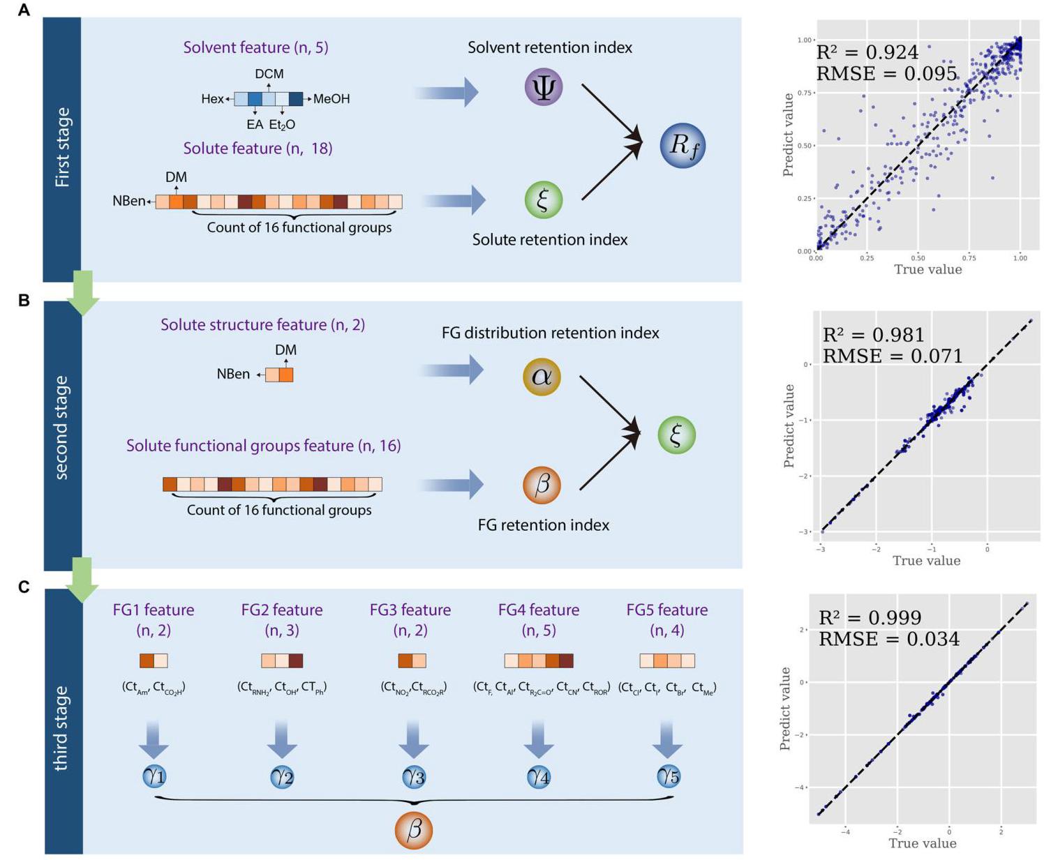
FIGURE 5 | Hierarchical structure of learning latent variables. Three stages are organized from top to bottom. (A) At the first stage, two latent variables, $\Psi$ and $\xi$ , are generated to encapsulate the overall polarity of the solvent and the solute, respectively. (B) At the second stage, two additional latent variables, $\alpha$ and $\beta$ , are learned to assess the solute molecule’s polarity from two distinct perspectives. $\alpha$ is linked to the distribution of functional groups, while $\beta$ pertains to the quantity of individual functional groups. (C) The third stage characterizes five latent variables, each representing the impact of specific groups of functional groups.
图5 | 学习潜在变量的层次结构。从顶部到底部组织了三个阶段。(A) 在第一阶段,生成两个潜在变量$\Psi$和$\xi$,分别封装溶剂和溶质的整体极性。(B) 在第二阶段,学习另外两个潜在变量$\alpha$和$\beta$,从两个不同的角度评估溶质分子的极性。$\alpha$与官能团的分布相关,而$\beta$与单个官能团的数量有关。(C) 第三阶段表征五个潜在变量,每个变量代表特定官能团组的影响。
DM (Dipole Moment): The dipole moment is a critical descriptor as it reflects the overall polarity of a molecule, indicating how electron density is distributed. However, the dipole moment alone might not fully capture the complexity of molecular interactions, especially in varied solvent environments. Its exclusion does affect the model, but not to the extent that it could singularly determine all polarity-related interactions. We found that combining the dipole moment with other descriptors provided a more robust prediction.
偶极矩(DM):偶极矩是一个关键描述符,因为它反映了分子的整体极性,表明电子密度的分布情况。然而,仅偶极矩可能无法完全捕捉分子相互作用的复杂性,特别是在不同的溶剂环境中。排除它确实会影响模型,但不至于仅凭它就能单独确定所有与极性相关的相互作用。我们发现将偶极矩与其他描述符结合起来能提供更可靠的预测。
NBen (Number of Benzene Ring): The presence and number of aromatic rings significantly influence molecular properties and interactions, particularly in aromatic-aromatic stacking and van der Waals interactions. These factors are crucial in many solute-solvent interactions that the dipole moment alone may not account for. In terms of features related to the solvent, we considered the volume ratios $\left( {V\% }\right)$ of five different solvent compounds, i.e., $n$ -hexane, ethyl acetate, dichloromethane, diethyl ether, and methanol.
苯环数(NBen):芳环的存在和数量对分子性质和相互作用有显著影响,特别是在芳环 - 芳环堆积和范德华相互作用中。这些因素在许多溶质 - 溶剂相互作用中至关重要,仅偶极矩可能无法解释这些相互作用。在与溶剂相关的特征方面,我们考虑了五种不同溶剂化合物的体积比$\left( {V\% }\right)$,即$n$ - 己烷、乙酸乙酯、二氯甲烷、乙醚和甲醇。
We conducted an input feature control experiment to evaluate the representation power of various feature sets. Two baseline feature sets were compared: one-hot encoded categorical features and random features. One-hot encoded features represent input features as binary vectors, where each postion indicates the presence or absence of a specific molecule. Random features, on the other hand, are randomly generated numerical values assigned to each molecule, serving as a non-informative baseline. In addition, we tested another two types of features commonly used in statistical models: 167D MACCS keys and conventional physicochemical descriptors. Specifically, these descriptors include molecular weight (MW), topological polar surface area (TPSA), the logarithm of $n$ -octanol-water partition coefficient (LogP), hydrogen bond donor number (HBD), hydrogen bond acceptor number (HBA), molecular polarity index (MPI), polar surface area percentage (PSA) and dipole moment (DM).
我们进行了一项输入特征控制实验,以评估各种特征集的表示能力。比较了两个基线特征集:独热编码分类特征和随机特征。独热编码特征将输入特征表示为二进制向量,其中每个位置表示特定分子的存在或不存在。另一方面,随机特征是为每个分子随机生成的数值,作为无信息基线。此外,我们测试了统计模型中常用的另外两种特征:167D MACCS键和传统物理化学描述符。具体来说,这些描述符包括分子量(MW)、拓扑极性表面积(TPSA)、$n$-辛醇-水分配系数的对数(LogP)、氢键供体数(HBD)、氢键受体数(HBA)、分子极性指数(MPI)、极性表面积百分比(PSA)和偶极矩(DM)。
A reaction
一个反应
component
组件
chemical-intuitive features [total length d=23]
化学直观特征 [总长度 d = 23]
solute (n=387) solvent (n=5)
溶质(n = 387) 溶剂(n = 5)
e.g. FG counts,
例如,官能团计数,
[1 .000, 1.408, 0.000, … 0.980, 0.0196, 0.000]
dipole moment
偶极矩
solute molecule features solvent features
溶质分子特征 溶剂特征
random features (k=18) (k=5)
随机特征 (k=18) (k=5)
[total length d =23]
[总长度d = 23]
k random features
k个随机特征
[0.374, 0.950 0.731 … -0.411, 1.021, 0.000]
for each unique molecule
对于每个独特的分子
mol. 1 mol.2 mol. 3 sol.3 sol.4 sol.5
分子1 分子2 分子3 溶剂3 溶剂4 溶剂5
one-hot encoding 1 0 0 … 1 0 0 ]
独热编码[1 0 0 … 1 0 0 ]
[total length d =392] 0 1 0 … 0 1 0 ]
[总长度d = 392][0 1 0 … 0 1 0 ]
n features for each 0 0 1 …
每个分子的n个特征
0 0 1 ]
molecule
分子
| B | Lin.Reg. | PLS | k-NN | NN | RF | Xgboost | |
| chemical-intuitive features | ${\mathbf{R}}^{2}$ | 0.666 | 0.654 | 0.686 | 0.874 | 0.849 | 0.938 |
| RMSE | 0.191 | 0.194 | 0.185 | 0.117 | 0.082 | 0.082 | |
| random features | ${\mathbf{R}}^{2}$ | 0.292 | 0.238 | 0.299 | 0.566 | 0.498 | 0.583 |
| RMSE | 0.278 | 0.288 | 0.276 | 0.217 | 0.234 | 0.213 | |
| one-hot encoding | ${\mathbf{R}}^{2}$ | 0.619 | 0.482 | 0.343 | 0.696 | 0.443 | 0.564 |
| RMSE | 0.204 | 0.238 | 0.268 | 0.210 | 0.246 | 0.218 | |
| MACCS [total length d=172] | ${\mathbf{R}}^{2}$ | 0.749 | 0.544 | 0.570 | 0.916 | 0.905 | 0.935 |
| RMSE | 0.165 | 0.223 | 0.216 | 0.095 | 0.103 | 0.084 | |
| physicochemical features [total length =13] | ${\mathbf{R}}^{2}$ | 0.608 | 0.574 | 0.525 | 0.606 | 0.887 | 0.950 |
| RMSE | 0.207 | 0.215 | 0.227 | 0.207 | 0.110 | 0.073 |
FIGURE 6 | Comparison of input feature control experiments. (A) Schematic of our features vs. random features and one-hot encoded categorical features. (B) Comparison of coefficient of determination $\left( {R}^{2}\right)$ and RMSE values between input features.
图6 | 输入特征控制实验的比较。(A) 我们的特征与随机特征和独热编码分类特征的示意图。(B) 输入特征之间的决定系数$\left( {R}^{2}\right)$和RMSE值的比较。
The five sets of input features were tested on six different machine learning models, including linear regression (Lin. Reg.), partial least squares (PLS), k-nearest neighbors (kNN), a simple neural network (NN), random forest (RF) and XGBoost. The results are presented in Figure 6.
这五组输入特征在六个不同的机器学习模型上进行了测试,包括线性回归(Lin. Reg.)、偏最小二乘法(PLS)、k近邻(kNN)、简单神经网络(NN)、随机森林(RF)和XGBoost。结果如图6所示。
3.2.2 | Architecture Design of Modular Neural Network
3.2.2 | 模块化神经网络的架构设计
The architecture of our network was motivated by the rationale grounded in established practices observed in TLC experiments. TLC experiments conventionally entailed the execution of controlled experiments designed to meticulously dissect the influence of solute polarity and solvent polarity on ${R}_{f}$ . To meet the specific demands of this task, we modified conventional Multi-Layer Perceptron (MLP) architecture into a modular neural network, designed to enhance interpretability and align with domain knowledge.
我们网络的架构是基于在TLC实验中观察到的既定实践原理。传统的TLC实验需要进行对照实验,旨在精心剖析溶质极性和溶剂极性对${R}_{f}$的影响。为了满足这项任务的特定需求,我们将传统的多层感知器(MLP)架构修改为模块化神经网络,旨在提高可解释性并与领域知识保持一致。
Feature Grouping. Let us consider a specific modular neural network. Given an input sample $\mathbf{x} \in {\mathbf{R}}^{d}$ , the initial step involved dividing the input features into $k$ feature groups, denoted as ${\mathbf{x}}_{1},\ldots ,{\mathbf{x}}_{k}$ . Each feature group ${\mathbf{x}}_{i} \in {\mathbf{R}}^{{d}_{i}}$ was non-overlapping, and their combined dimensionality satisfied $\mathop{\sum }\limits_{{i = 1}}^{k}{d}_{i} = d$ . These feature groups were determined using a chemist-guided strategy, and the specific grouping applied at each stage is illustrated in Figure 5. Specifically, in the first stage, we categorized features into two distinct groups: solvent features $\left( {{\mathbf{x}}_{\text{ solvent }} \in {\mathbf{R}}^{5}}\right)$ and solute features $\left( {{\mathbf{x}}_{\text{ solute }} \in {\mathbf{R}}^{18}}\right)$ . In the second stage, the solute features were further categorized into two groups: FG features $\left( {{\mathbf{x}}_{\mathrm{{FG}}} \in {\mathbf{R}}^{16}}\right)$ and FG distribution features $\left( {{\mathbf{x}}_{\text{ FGdist }} \in {\mathbf{R}}^{2}}\right)$ . In the third stage, the FG features were further categorized into five distinct groups: ${\mathbf{x}}_{\mathrm{{FG}}1} \in {\mathbf{R}}^{2},{\mathbf{x}}_{\mathrm{{FG}}2} \in {\mathbf{R}}^{3},{\mathbf{x}}_{\mathrm{{FG}}3} \in {\mathbf{R}}^{2},{\mathbf{x}}_{\mathrm{{FG}}4} \in {\mathbf{R}}^{5}$ and ${\mathbf{x}}_{\mathrm{{FG}}5} \in {\mathbf{R}}^{4}$ .
特征分组。让我们考虑一个特定的模块化神经网络。给定一个输入样本$\mathbf{x} \in {\mathbf{R}}^{d}$,初始步骤涉及将输入特征划分为$k$个特征组,记为${\mathbf{x}}_{1},\ldots ,{\mathbf{x}}_{k}$。每个特征组${\mathbf{x}}_{i} \in {\mathbf{R}}^{{d}_{i}}$不重叠,并且它们的组合维度满足$\mathop{\sum }\limits_{{i = 1}}^{k}{d}_{i} = d$。这些特征组是使用化学家指导的策略确定的,每个阶段应用的具体分组如图5所示。具体来说,在第一阶段,我们将特征分为两个不同的组:溶剂特征$\left( {{\mathbf{x}}_{\text{ solvent }} \in {\mathbf{R}}^{5}}\right)$和溶质特征$\left( {{\mathbf{x}}_{\text{ solute }} \in {\mathbf{R}}^{18}}\right)$。在第二阶段,溶质特征进一步分为两组:FG特征$\left( {{\mathbf{x}}_{\mathrm{{FG}}} \in {\mathbf{R}}^{16}}\right)$和FG分布特征$\left( {{\mathbf{x}}_{\text{ FGdist }} \in {\mathbf{R}}^{2}}\right)$。在第三阶段,FG特征进一步分为五个不同的组:${\mathbf{x}}_{\mathrm{{FG}}1} \in {\mathbf{R}}^{2},{\mathbf{x}}_{\mathrm{{FG}}2} \in {\mathbf{R}}^{3},{\mathbf{x}}_{\mathrm{{FG}}3} \in {\mathbf{R}}^{2},{\mathbf{x}}_{\mathrm{{FG}}4} \in {\mathbf{R}}^{5}$和${\mathbf{x}}_{\mathrm{{FG}}5} \in {\mathbf{R}}^{4}$。
Latent Representation and Modularity. A key innovation of our architecture lay in the formulation of the target latent representation layer $j$ , where ${z}_{i}^{\left( j\right) } = {g}_{i}\left( {\mathbf{x}}_{i}\right)$ . Each function ${g}_{i}$ operated independently within the modular neural network, meaning there was no parameter sharing across ${g}_{1},\ldots ,{g}_{k}$ . Thus, we could consider ${g}_{i}$ as a sub-model. This design ensured the preservation of feature-specific information. The final output, $o = h\left( {\mathbf{z}}^{\left( j\right) }\right)$ , encapsulated the information from the target latent representation layer.
潜在表示与模块化。我们架构的一个关键创新在于目标潜在表示层$j$的公式化,其中${z}_{i}^{\left( j\right) } = {g}_{i}\left( {\mathbf{x}}_{i}\right)$。每个函数${g}_{i}$在模块化神经网络中独立运行,这意味着在${g}_{1},\ldots ,{g}_{k}$之间没有参数共享。因此,我们可以将${g}_{i}$视为一个子模型。这种设计确保了特定特征信息的保留。最终输出$o = h\left( {\mathbf{z}}^{\left( j\right) }\right)$封装了来自目标潜在表示层的信息。
This design restricted the receptive field of the latent variables, therefore ensuring that each latent variable depended solely on a specific group of input features. For instance, in the first stage, the latent variables learned from solvent features and solute features were interpreted as the solvent retention index $\left( \Psi \right)$ and the solute retention index $\left( \xi \right)$ , respectively. These indices captured distinct contributions from the input features, reflecting their individual effects on ${R}_{f}$ .
这种设计限制了潜在变量的感受野,因此确保每个潜在变量仅依赖于特定的一组输入特征。例如,在第一阶段,从溶剂特征和溶质特征学习到的潜在变量分别被解释为溶剂保留指数$\left( \Psi \right)$和溶质保留指数$\left( \xi \right)$。这些指数捕获了输入特征的不同贡献,反映了它们对${R}_{f}$的各自影响。
Training Procedure. The training procedure consisted of three stages, with each stage involving a modular neural network to extract retention indices that reflected different levels of granularity, as illustrated in Figure 5. In the first stage, the input features were divided into two feature groups: solvent features and solute features. These were processed independently by the modular neural network, resulting in two latent variables: the solvent retention index $\left( \Psi \right)$ and the solute retention index $\left( \xi \right)$ . These indices represented the overall contributions of solvent and solute features to the ${R}_{f}$ value.
训练过程。训练过程包括三个阶段,每个阶段都涉及一个模块化神经网络,用于提取反映不同粒度水平的保留指数,如图5所示。在第一阶段,输入特征被分为两个特征组:溶剂特征和溶质特征。这些特征由模块化神经网络独立处理,产生两个潜在变量:溶剂保留指数$\left( \Psi \right)$和溶质保留指数$\left( \xi \right)$。这些指数代表了溶剂和溶质特征对${R}_{f}$值的总体贡献。
In the second stage, we focused on solute features only. The solute features were further divided into two subgroups: functional group (FG) counts and the distribution of functional groups within the molecule. The modular neural network processed these subgroups to extract two additional indices: the FG retention index $\left( \beta \right)$ , which captured the contribution of different FGs to ${R}_{f}$ , and the FG distribution retention index $\left( \alpha \right)$ , which represented the influence of how functional groups were distributed across the molecule. These indices provided a more detailed understanding of how functional groups impact molecular polarity and retention behavior.
在第二阶段,我们仅关注溶质特征。溶质特征进一步分为两个子组:官能团(FG)计数和分子内官能团的分布。模块化神经网络处理这些子组以提取另外两个指数:FG保留指数$\left( \beta \right)$,它捕获了不同FG对${R}_{f}$的贡献,以及FG分布保留指数$\left( \alpha \right)$,它代表了官能团在分子中分布方式的影响。这些指数提供了对官能团如何影响分子极性和保留行为的更详细理解。
The third stage involved a fine-grained analysis of functional group contributions. Here, the FG features were further subdivided into five specific FG categories. Using the modular neural network, five fine-grained FG retention indices $\left( {{\gamma }_{1},\ldots ,{\gamma }_{5}}\right)$ were extracted. These FG retention indices captured the unique contributions of specific types of functional groups to ${R}_{f}$ .
第三阶段涉及对官能团贡献的细粒度分析。在这里,FG特征进一步细分为五个特定的FG类别。使用模块化神经网络,提取了五个细粒度的FG保留指数$\left( {{\gamma }_{1},\ldots ,{\gamma }_{5}}\right)$。这些FG保留指数捕获了特定类型的官能团对${R}_{f}$的独特贡献。
This hierarchical decomposition, progressing from broad solvent and solute features to detailed FG-specific contributions, ensured that the model disentangles complex relationships between molecular features and the ${R}_{f}$ value.
这种从宽泛的溶剂和溶质特征到详细的FG特定贡献的层次分解,确保了模型能够解开分子特征与${R}_{f}$值之间的复杂关系。
3.2.3 | Symbolic Regression
3.2.3 | 符号回归
SR aims to identify mathematical expressions that capture the inherent relationships within a given dataset. Unlike approaches that involve fitting parameters to overly complex general models (such as machine learning models), SR explores a space of simple analytic expressions. The goal is to discover accurate and explainable models that directly represent the underlying patterns in the data. SR is usually implemented by evolutionary algorithms, such as genetic programming (GP) $\left\lbrack {{29},{30},{48}}\right\rbrack$ .
符号回归旨在识别能够捕捉给定数据集中内在关系的数学表达式。与那些将参数拟合到过于复杂的通用模型(如机器学习模型)的方法不同,符号回归探索的是简单解析表达式的空间。其目标是发现能够直接表示数据中潜在模式的准确且可解释的模型。符号回归通常由进化算法实现,如遗传编程(GP)$\left\lbrack {{29},{30},{48}}\right\rbrack$ 。
The most common way to visualize a symbolic expression is a tree-structure with nodes and branches, as shown in Figure 3A. This structure includes primitive functions (e.g., $+ , - , \times , \div ,$ exp) and terminal nodes (input features and numeric constants). Through a series of mutation operations, the GP algorithm seeks to determine the optimal number of nodes and terminals that provide the best fit to a given dataset. For our implementation of the widely used GP-SR algorithm, we employed the open-source Python library PySR ${}^{1}$ [49]. The hyperparameter configurations for our implementation are detailed in the Tables S8 and S9. Moreover, when deriving the ${R}_{f}$ governing equations, we imposed a constraint requiring all parameters to be positive. If any parameter turned out to be negative, we added a minus sign before the learned retention index to standardize the results.
可视化符号表达式最常见的方式是使用带有节点和分支的树形结构,如图3A所示。这种结构包括基本函数(例如,$+ , - , \times , \div ,$ exp)和终端节点(输入特征和数值常量)。通过一系列变异操作,GP算法试图确定能最佳拟合给定数据集的节点和终端的最佳数量。对于我们实现的广泛使用的GP - SR算法,我们采用了开源Python库PySR ${}^{1}$ [49]。我们实现的超参数配置在表S8和S9中有详细说明。此外,在推导${R}_{f}$ 控制方程时,我们施加了一个约束,要求所有参数为正。如果任何参数结果为负,我们在学习到的松香指数前添加一个负号以使结果标准化。
It is worth mentioning that our method is not limited to GP algorithms. In fact, the UHSR framework is designed to accommodate various symbolic regression methods; comparable results obtained from deep reinforcement learning based SR methods (such as DISCOVER ${}^{2}$ [50]) are included in the Table S5.
值得一提的是,我们的方法不限于GP算法。事实上,UHSR框架旨在适应各种符号回归方法;基于深度强化学习的SR方法(如DISCOVER ${}^{2}$ [50])获得的可比结果包含在表S5中。
3.3 | Expert Chemist Evaluation
3.3 | 专家化学家评估
The expert chemist evaluation consists of a quantitative survey assessment in which chemists were provided with a QR code or website link to complete the survey (please see Supporting Information for the complete survey). The study was submitted for ethical review and received approval from the Peking University Institutional Review Board (No. IRB00001052-2408). Participation was not incentivized with compensation, as it was considered to contribute to the general advancement of research. The study was anonymous, and only the lead researcher had access to the assignment of the experimental IDs. Participants were chemical professionals, including faculty members, industry chemists, and graduate students, representing a wide range of experiences and roles in chemistry-related fields (Please see Figure S3 for geographic statistics of the participants). This survey aimed to evaluate the chemists’ opinions on the interpretability of the UHSR model vs. traditional machine learning models. Participants provided their feedback based on their professional experience, and demographic data such as years of experience, educational background, and geographical region were collected to ensure a comprehensive analysis. A total of 101 chemists agreed to participate. One response was excluded due to an invalid answer, leaving 100 valid responses.
专家化学家评估包括一项定量调查评估,在此评估中,为化学家提供了二维码或网站链接以完成调查(完整调查请见补充信息)。该研究已提交伦理审查并获得北京大学机构审查委员会的批准(编号IRB00001052 - 2408)。参与研究未给予报酬激励,因为认为这有助于推动研究的总体进展。该研究是匿名的,只有首席研究员有权访问实验ID的分配。参与者为化学专业人士,包括教职员工、行业化学家以及研究生,他们在化学相关领域代表了广泛的经验和角色(参与者的地理统计信息请见图S3)。本次调查旨在评估化学家对UHSR模型与传统机器学习模型可解释性的看法。参与者根据其专业经验提供反馈,并收集了诸如工作年限、教育背景和地理区域等人口统计数据,以确保进行全面分析。共有101位化学家同意参与。由于一个无效答案,排除了一份回复,最终得到100份有效回复。
3.4 | Experimental Settings and Training Details
<### 3.4 | 实验设置与训练细节
When constructing the modular neural network, at each stage, we set the number of neurons in the hidden layers of each sub-model to 50. Furthermore, two hidden layers were employed. To facilitate the discovery of concise equations, we leaned toward employing a relatively simple network structure, which helps to prevent overfitting to experimental noise. The activation function chosen for each sub-model was LeakyReLU. In the first stage, the activation function of the output layer was set to a sigmoid, which ensures a standardized output within the range of 0 and 1 (Figure 3B). The batch size was set to 2048, and the Adam optimizer implemented in PyTorch was applied. The learning rate was 0.01 .
在构建模块化神经网络时,在每个阶段,我们将每个子模型隐藏层中的神经元数量设置为50。此外,使用了两个隐藏层。为了便于发现简洁的方程,我们倾向于采用相对简单的网络结构,这有助于防止过度拟合实验噪声。为每个子模型选择的激活函数是LeakyReLU。在第一阶段,输出层的激活函数设置为sigmoid,这确保了在0到1范围内的标准化输出(图3B)。批量大小设置为2048,并应用了PyTorch中实现的Adam优化器。学习率为0.01。
${}^{1}$ https://github.com/MilesCranmer/PySR
${}^{1}$ https://github.com/MilesCranmer/PySR
${}^{2}$ https://github.com/menggedu/DISCOVER
${}^{2}$ https://github.com/menggedu/DISCOVER
To evaluate the performance and generalizability of UHSR, we employed 10-fold cross-validation. The full dataset was randomly partitioned into 10 equal subsets. For each fold, 9 folds were used to train the model, and the remaining fold was used for testing. This process was repeated 10 times, ensuring that each data point was used for both training and testing. Each modular neural network was trained for 1000 epochs, then the best validation checkpoint was selected for testing. We conducted the evaluation in two parts: the modular neural networks to produce retention indices, and the derived ${R}_{f}$ equations.
为了评估UHSR的性能和泛化能力,我们采用了10折交叉验证。完整的数据集被随机划分为10个相等的子集。对于每一折,使用9折来训练模型,其余一折用于测试。这个过程重复10次,确保每个数据点都用于训练和测试。每个模块化神经网络训练1000个轮次,然后选择最佳的验证检查点进行测试。我们分两部分进行评估:模块化神经网络以生成保留指数,以及导出的${R}_{f}$方程。
The performance of the modular neural networks was evaluated in each fold using the $R$ -squared coefficient $\left( {R}^{2}\right)$ and the root mean square error (RMSE), which are defined as
在每一折中,使用$R$ -平方系数$\left( {R}^{2}\right)$和均方根误差(RMSE)来评估模块化神经网络的性能,它们的定义如下
$$ {R}^{2} = 1 - \frac{\mathop{\sum }\limits_{{i = 1}}^{N}{\left( {y}_{i} - {\widehat{y}}_{i}\right) }^{2}}{\mathop{\sum }\limits_{{i = 1}}^{N}{\left( {y}_{i} - \bar{y}\right) }^{2}},\;\text{ RMSE } = \sqrt{\frac{\mathop{\sum }\limits_{{i = 1}}^{N}{\left( {y}_{i} - {\widehat{y}}_{i}\right) }^{2}}{N}} $$where $N$ is the total number of samples, ${y}_{i}$ and ${\widehat{y}}_{i}$ represent the label and the prediction value for the $i$ -th sample, and $\bar{y}$ denotes the mean of the ground truth values.
其中$N$是样本总数,${y}_{i}$和${\widehat{y}}_{i}$分别表示第$i$个样本的标签和预测值,$\bar{y}$表示真实值的均值。
The results, presented in Table S2, demonstrate consistently high ${R}^{2}$ values and low RMSE values across all folds, indicating the robustness of the modular neural networks. We also derived the ${R}_{f}$ governing equations of each fold, as shown in Table S3. Most equations share a similar structure. Although the coefficients for $\Psi$ and $\xi$ vary slightly across folds, but generally remain within a consistent range.
表S2中呈现的结果表明,在所有折中,${R}^{2}$值始终很高,RMSE值很低,这表明模块化神经网络的稳健性。我们还导出了每一折的${R}_{f}$控制方程,如表S3所示。大多数方程具有相似的结构。尽管$\Psi$和$\xi$的系数在各折之间略有不同,但总体上仍保持在一致的范围内。
4 | Discussion and Conclusion
4 | 讨论与结论
Chellenges in current approaches to explainability. Recent efforts to establish quantitative structure-polarity relationships primarily rely on machine learning models and the development of informative feature representations [16, 23]. While these approaches achieve high prediction accuracy, a significant limitation lies in their lack of interpretability. This lack of transparency hinders a deeper understanding of the intrinsic relationships within the data, consequently reducing the scientific impact of these models by limiting researchers’ ability to trust and fully comprehend their predictions [26-28].
当前可解释性方法面临的挑战。近期建立定量结构 - 极性关系的努力主要依赖于机器学习模型和信息性特征表示的开发[16, 23]。虽然这些方法实现了高预测准确性,但一个重大限制在于它们缺乏可解释性。这种缺乏透明度阻碍了对数据内在关系的深入理解,从而通过限制研究人员信任和完全理解其预测的能力降低了这些模型的科学影响力[26 - 28]。
To address this challenge, explainable methods have been developed, broadly categorized into intrinsic and post-hoc approaches. Post-hoc methods, such as LIME [51] and Shapley values [52], provide insights into the importance of input variables relative to model outputs. However, these methods are limited in their ability to explain the model’s internal mechanisms, offering only a partial understanding of how features interact or contribute to predictions. They essentially provide a narrow view into the “black box,” revealing feature importance without elucidating the relationships that drive the model’s decisions. Conversely, intrinsic models, such as multiple linear regression or partial least squares, are inherently interpretable but often lack the accuracy required to handle complex datasets (Figure 6B).
为应对这一挑战,已开发出可解释性方法,大致分为内在方法和事后方法。事后方法,如LIME[51]和Shapley值[52],提供了关于输入变量相对于模型输出重要性的见解。然而,这些方法在解释模型内部机制方面能力有限,仅提供了对特征如何相互作用或对预测有贡献的部分理解。它们本质上提供了对“黑箱”的狭隘视角,揭示了特征重要性却未阐明驱动模型决策的关系。相反,内在模型,如多元线性回归或偏最小二乘法,本质上是可解释的,但往往缺乏处理复杂数据集所需的准确性(图6B)。
The UHSR framework introduced in this study offers an alternative solution. By integrating equation-based modeling with hierarchical insights into feature importance. Unlike traditional methods, UHSR not only identifies key features but also explains how these features interact and propagate through the hierarchical structure to influence the final output. Key to this framework are two retention indices, the solvent retention index $\left( \Psi \right)$ and the solute retention index $\left( \xi \right)$ . These indices provide interpretable insights into the structure-polarity relationship while enabling direct ${R}_{f}$ prediction through a formula-driven approach. By leveraging only a few indices (in this case, two) closely tied to the dataset, UHSR enhances interpretability and reduces complexity compared to high-dimensional feature representations. Moreover, the predictive accuracy of UHSR is comparable to that of existing DNN models, demonstrating that interpretability does not need to come at the cost of performance.
本研究中引入的UHSR框架提供了一种替代解决方案。通过将基于方程的建模与对特征重要性的层次化见解相结合。与传统方法不同,UHSR不仅识别关键特征,还解释这些特征如何通过层次结构相互作用和传播以影响最终输出。该框架的关键是两个保留指数,溶剂保留指数$\left( \Psi \right)$和溶质保留指数$\left( \xi \right)$。这些指数提供了对结构 - 极性关系的可解释见解,同时通过公式驱动的方法实现直接${R}_{f}$预测。通过仅利用与数据集紧密相关的几个指数(在这种情况下为两个),与高维特征表示相比,UHSR提高了可解释性并降低了复杂性。此外,UHSR的预测准确性与现有DNN模型相当,表明可解释性无需以性能为代价。
Advantages of UHSR beyond interpretability. The symbolic regression component of UHSR offers several notable advantages over traditional machine learning models, particularly for deployment in automated platforms and resource-constrained environments. (1) Deployment efficiency and low computational cost. Although the training cost of UHSR is higher than standard machine learning models due to the additional step of extracting interpretable equations, its key advantage lies in deployment efficiency. Once the symbolic equations are discovered, inference becomes nearly instantaneous, requiring only a few arithmetic operations. In contrast, black-box models like DNNs involve evaluating large numbers of parameters during inference, leading to significantly higher computational demands. This makes UHSR particularly advantageous for automated platforms, where real-time predictions with minimal computational overhead are critical. (2) Robustness and transferability. Equation-based models have fewer parameters compared to traditional machine learning models, resulting in improved robustness and transferability. These models are less prone to overfitting and can adapt to new conditions with minimal retraining. Unlike DNNs, which often require extensive fine-tuning and retraining when applied to new scenarios, symbolic equations derived from UHSR offer cost-effective adaptability while retaining interpretability.
UHSR除可解释性之外的优势。UHSR的符号回归组件相对于传统机器学习模型具有几个显著优势,特别是在自动平台和资源受限环境中的部署。(1) 部署效率和低计算成本。尽管由于提取可解释方程的额外步骤,UHSR的训练成本高于标准机器学习模型,但其关键优势在于部署效率。一旦发现符号方程,推理几乎瞬间完成,只需要几个算术运算。相比之下,像DNN这样的黑箱模型在推理过程中涉及评估大量参数,导致计算需求显著更高。这使得UHSR对于自动平台特别有利,在这些平台中,以最小的计算开销进行实时预测至关重要。(2) 鲁棒性和可转移性。基于方程的模型与传统机器学习模型相比参数更少,从而提高了鲁棒性和可转移性。这些模型不太容易过拟合,并且可以在几乎不需要重新训练的情况下适应新条件。与DNN不同,当应用于新场景时,DNN通常需要广泛的微调与重新训练,而从UHSR导出的符号方程在保持可解释性的同时提供了经济高效的适应性。
Current limitations and future directions. Despite these strengths, the current study has several limitations, which in turn represent exciting future directions. (1) Dataset Coverage. First, the UHSR model is restricted to the solvent systems represented in the TLC dataset. While the five solvents included are widely used in TLC experiments and adequately represent typical solvent systems (as indicated by 82.0% of surveyed chemists), the current framework cannot address more complex eluents with additives (e.g., AcOH or ${\mathrm{{NEt}}}_{3}$ ) or solvent systems beyond those represented in the dataset. Extending the framework to such systems would require incorporating additional experimental data and retraining the model on an expanded dataset. Second, the diversity of analytes in the training set is also limited, as it predominantly consists of substituted arenes and heteroarenes, which are rigid, planar scaffolds. These analytes’ retention behavior can be effectively captured by the chemically intuitive features developed in this study, such as functional group counts and a single orientation descriptor. However, this limits the model’s applicability to more diverse molecular structures. For example, heterocycles without benzene rings (e.g., thiophene, pyridine) or molecules with multiple benzene rings and fused rings (e.g., naphthalene) would require the introduction of additional chemically intuitive features, such as pyridine nitrogen, thiophene sulfur, fused ring descriptors, or steroid core types. While the current framework is not yet equipped to handle these cases, its flexibility allows for adaptation to new molecular classes once the dataset is expanded. Third, the model’s focus on analytes that are predominantly ${\mathrm{{sp}}}^{2}$ - rich. The chemically intuitive features developed in this study may not generalize well to conformationally flexible, ${\mathrm{{sp}}}^{3}$ -rich molecules, even if they share similar functional groups. Future work will address this limitation by enriching the dataset with diverse 3D scaffolds and developing feature sets that incorporate 3D descriptors (e.g., conformer-ensemble statistics, dihedral angle distributions, and 3D autocorrelation functions). These efforts will help maintain the symbolic regression framework’s interpretability while extending its applicability to a broader range of chemical structures.
当前的局限性和未来方向。尽管有这些优势,但本研究仍有若干局限性,这些局限性反过来也代表了令人兴奋的未来方向。(1) 数据集覆盖范围。首先,UHSR模型仅限于TLC数据集中所代表的溶剂体系。虽然所包含的五种溶剂在TLC实验中广泛使用,并充分代表了典型的溶剂体系(82.0%的受访化学家表示如此),但当前框架无法处理含有添加剂(如AcOH或${\mathrm{{NEt}}}_{3}$)的更复杂洗脱液或数据集中未涵盖的溶剂体系。将框架扩展到此类体系需要纳入额外的实验数据,并在扩展数据集上重新训练模型。其次,训练集中分析物的多样性也有限,因为它主要由取代芳烃和杂芳烃组成,这些都是刚性的平面骨架。本研究中开发的化学直观特征,如官能团计数和单一取向描述符,可以有效地捕捉这些分析物的保留行为。然而,这限制了模型对更多样化分子结构的适用性。例如,没有苯环的杂环(如噻吩、吡啶)或具有多个苯环和稠环的分子(如萘)将需要引入额外的化学直观特征,如吡啶氮、噻吩硫、稠环描述符或甾体核心类型。虽然当前框架尚不具备处理这些情况的能力,但其灵活性允许在数据集扩展后适应新的分子类别。第三,模型主要关注富含${\mathrm{{sp}}}^{2}$的分析物。本研究中开发的化学直观特征可能无法很好地推广到构象灵活、富含${\mathrm{{sp}}}^{3}$的分子,即使它们具有相似的官能团。未来的工作将通过用多样的3D支架丰富数据集,并开发纳入3D描述符(如构象体统计、二面角分布和3D自相关函数)的特征集来解决这一局限性。这些努力将有助于在保持符号回归框架可解释性的同时,将其适用性扩展到更广泛的化学结构范围。
(2) Non-Uniqueness of Derived Equations. It is important to note that the retention indices and governing equations derived from the UHSR model are not unique solutions. Due to the inherent limitations of the data, different neural networks (and their corresponding equations) can achieve similar levels of accuracy (see Tables S10-S12 for details). This phenomenon is common in scientific discovery, where multiple models can explain observed phenomena equally well. For example, in reaction kinetics, different rate laws derived from experimental data often describe the same behavior. UHSR is designed to provide one interpretable solution to the problem, aiming to enhance understanding and inspire further research within the field.
(2) 导出方程的非唯一性。需要注意的是,从UHSR模型导出的保留指数和控制方程不是唯一解。由于数据的固有局限性,不同的神经网络(及其相应的方程)可以达到相似的准确度水平(详细信息见表格S10 - S12)。这种现象在科学发现中很常见,即多个模型可以同样好地解释观察到的现象。例如,在反应动力学中,从实验数据导出的不同速率定律通常描述相同的行为。UHSR旨在为该问题提供一个可解释的解决方案,旨在增进理解并激发该领域内进一步的研究。
(3) Reliance on prior knowledge for feature selection and grouping. The current implementation of the UHSR framework relies heavily on expert-defined feature selection and grouping strategies, which were used to construct the solvent retention index $\left( \Psi \right)$ and solute retention index $\left( \xi \right)$ . While this approach ensures that the derived equations are chemically meaningful and interpretable, it introduces a dependency on prior chemical knowledge. This limits the scalability of the framework, particularly when applied to novel chemical spaces or datasets with less defined chemical properties. Future work will explore more automated approaches to feature selection and grouping to reduce reliance on domain expertise. For instance, unsupervised learning methods such as clustering molecular descriptors could be employed to identify functional groups or suggest feature groupings in a data-driven manner.
(3) 在特征选择和分组上对先验知识的依赖。UHSR框架的当前实现严重依赖专家定义的特征选择和分组策略,这些策略用于构建溶剂保留指数$\left( \Psi \right)$和溶质保留指数$\left( \xi \right)$。虽然这种方法确保导出的方程在化学上有意义且可解释,但它引入了对先验化学知识的依赖。这限制了框架的可扩展性,特别是当应用于新颖的化学空间或化学性质定义较少的数据集时。未来的工作将探索更自动化的特征选择和分组方法,以减少对领域专业知识的依赖。例如,可以采用无监督学习方法,如聚类分子描述符,以数据驱动的方式识别官能团或建议特征分组。
Broader implications. While this study focuses on applications in chemistry, the development of explainable frameworks has broader relevance. By improving the interpretability of machine learning models, our framework can enhance trust in predictions and foster collaboration across scientific disciplines, contributing to advancements in data-driven discovery.
更广泛的意义。虽然本研究侧重于化学领域的应用,但可解释框架的开发具有更广泛的相关性。通过提高机器学习模型的可解释性,我们的框架可以增强对预测的信任,并促进跨科学学科的合作,为数据驱动的发现做出贡献。
Acknowledgements
致谢
We thank the National Natural Science Foundation of China (Grant No. 12572266) and the New Generation Artificial Intelligence-National Science and Technology Major Project (grant no. 2025ZD0121904). We also thank the High Performance Computing Platform of Peking University and the High Performance Computing Centers at Eastern Institute of Technology, Ningbo, for machine learning model training. We also thank Mengge Du for assisting in the implementation of DISCOVER. [Correction added on 5-February-2026, after first online publication: New funder is added in the acknowledgment section.]
我们感谢中国国家自然科学基金(项目编号:12572266)以及新一代人工智能国家科技重大专项(项目编号:2025ZD0121904)。我们还感谢北京大学高性能计算平台以及宁波东方理工大学高性能计算中心为机器学习模型训练提供支持。我们也感谢杜梦歌协助实施DISCOVER。[2026年2月5日首次在线发表后添加的更正:致谢部分新增了资助机构。]
Ethics Statement Heading
伦理声明标题
The survey conducted in the study was submitted for ethical review and received approval from the Peking University Institutional Review Board, No. IRB00001052-2408.
本研究中进行的调查已提交伦理审查,并获得北京大学机构审查委员会(编号:IRB00001052 - 2408)的批准。
Conflicts of Interest
利益冲突
The authors declare no conflicts of interest.
作者声明不存在利益冲突。
Data Availability Statement
数据可用性声明
The original code for the experiments and data analysis in this work has been deposited at the website: https://github.com/SiyuLou/ UnsupervisedHierarchicalSymbolicRegression
本研究中实验和数据分析的原始代码已存放在网站:https://github.com/SiyuLou/UnsupervisedHierarchicalSymbolicRegression
References
参考文献
H. W. de Regt, Understanding Scientific Understanding (Oxford University Press, 2017).
A. Potochnik, Idealization and the Aims of Science (University of Chicago Press, 2017).
W. Henry and J. Banks, “Iii. Experiments on the Quantity of Gases Absorbed by Water, at Different Temperatures, and under Different Pressures,” Philosophical Transactions of the Royal Society A: Mathematical, Physical and Engineering Sciences 93 (1803): 29-274.
S. Arrhenius, “Über Die Reaktionsgeschwindigkeit Bei Der Inversion Von Rohrzucker Durch Säuren,” Zeitschrift für physikalische Chemie 4, no. 1 (1889): 226-248.
J. H. van’t Hoff, Études de Dynamique Chimique (F. Muller & Co., Amsterdam, 1884).
G. M. Sessler, Physical Principles of Electrets (Springer, Berlin, Heidelberg, 1987), https://doi.org/10.1007/3540173358_10.
A. R. Katritzky, D. C. Fara, H. Yang, K. Tämm, T. Tamm, and M. Karelson, “Quantitative Measures of Solvent Polarity,” Chemical Reviews 104, no. 1 (2004): 175-198.
M. H. Abraham, A. Ibrahim, and A. M. Zissimos, “Determination of Sets of Solute Descriptors from Chromatographic Measurements,” Journal of Chromatography A 1037, no. 1-2 (2004): 29-47.
C. F. Poole, “Reversed-Phase Liquid Chromatography System Constant Database over an Extended Mobile Phase Composition Range for 25 Siloxane-Bonded Silica-Based Columns,” Journal of Chromatography A 1600 (2019): 112-126.
C. F. Poole and N. Lenca, “Reversed-Phase Liquid Chromatography,” in Liquid Chromatography (Elsevier, 2017), pp. 91-123.
U. D. Neue and H.-J. Kuss, “Improved Reversed-Phase Gradient Retention Modeling,” Journal of Chromatography A 1217, no. 24 (2010): 3794-3803.
K. Ciura, S. Dziomba, J. Nowakowska, and M. J. Markuszewski, “Thin Layer Chromatography in Drug Discovery Process,” Journal of Chromatography A 1520 (2017): 9-22.
C. F. Poole, “Thin-Layer Chromatography: Challenges and Opportunities,” Journal of Chromatography A 1000, no. 1 (2003): 963-984.
Ł. Komsta, “A Functional-Based Approach to the Retention in Thin Layer Chromatographic Screening Systems,” Analytica Chimica Acta 629, no. 1 (2008): 66-72, https://doi.org/10.1016/j.aca.2008.09.036.
S. Yousefinejad, F. Honarasa, and N. Saeed, “Quantitative Structure-Retardation Factor Relationship of Protein Amino Acids in Different Solvent Mixtures for Normal-Phase Thin-Layer Chromatography,” Journal of Separation Science 38, no. 10 (2015): 1771-1776.
H. Xu, J. Lin, Q. Liu, et al., “High-Throughput Discovery of Chemical Structure-Polarity Relationships Combining Automation and Machine-Learning Techniques,” Chem 8, no. 12 (2022): 3202-3214, https://doi.org/ 10.1016/j.chempr.2022.08.008.
H. Xu, D. Zhang, and F. Mo, “High-Throughput Automated Platform for Thin Layer Chromatography Analysis,” STAR Protocols 3, no. 4 (2022): 101893.
A. F. Zahrt, J. J. Henle, B. T. Rose, Y. Wang, W. T. Darrow, and S. E. Denmark, “Prediction of Higher-Selectivity Catalysts by Computer-Driven Workflow and Machine Learning,” Science 363, no. 6424 (2019): eaau5631, https://doi.org/10.1126/science.aau5631.
E. N. Muratov, J. Bajorath, R. P. Sheridan, et al., “Qsar Without Borders,” Chemical Society Reviews 49, no. 11 (2020): 3525-3564.
C. B. Wahl, M. Aykol, J. H. Swisher, J. H. Montoya, S. K. Suram, and C. A. Mirkin, “Machine Learning-Accelerated Design and Synthesis of Polyelemental Heterostructures,” Science Advances 7, no. 52 (2021): eabj5505, https://doi.org/10.1126/sciadv.abj5505.
N. I. Rinehart, R. K. Saunthwal, J. Wellauer, et al., “A Machine-Learning Tool to Predict Substrate-Adaptive Conditions for Pd-Catalyzed C-N Couplings,” Science 381, no. 6661 (2023): 965-972, https://doi.org/10.1126/science.adg2114.
J. Lin, H. Zhang, M. Asadi, et al., “Machine Learning-Driven Discovery and Structure-Activity Relationship Analysis of Conductive MetalOrganic Frameworks,” Chemistry of Materials 36, no. 11 (2024): 5436-5445, https://doi.org/10.1021/acs.chemmater.4c00229.
Q. Yang, Y. Li, J.-D. Yang, et al., “Holistic Prediction of the Pka in Diverse Solvents Based on a Machine-Learning Approach,” Angewandte Chemie International Edition 59, no. 43 (2020): 19282-19291, https://doi.org/10.1002/anie.202008528.
Y. Yao, Q. Dong, A. Brozena, et al., “High-Entropy Nanoparticles: Synthesis-Structure-Property Relationships and Data-Driven Discovery,” Science 376, no. 6589 (2022): eabn3103, https://doi.org/10.1126/science.abn3103.
B. A. Koscher, R. B. Canty, M. A. McDonald, et al., “Autonomous, Multiproperty-Driven Molecular Discovery: From Predictions to Measurements and Back,” Science 382, no. 6677 (2023): eadi1407, https://doi.org/10.1126/science.adi1407.
C. Rudin, “Stop Explaining Black Box Machine Learning Models for High Stakes Decisions and Use Interpretable Models Instead,” Nature Machine Intelligence 1, no. 5 (2019): 206-215.
R. Geirhos, J.-H. Jacobsen, C. Michaelis, et al., “Shortcut Learning in Deep Neural Networks,” Nature Machine Intelligence 2, no. 11 (2020): 665- 673.
Z. C. Lipton, “The Mythos of Model Interpretability: In Machine Learning, the Concept of Interpretability Is Both Important and Slippery,” Queue 16, no. 3 (2018): 31-57.
L. Billard and E. Diday, “From the Statistics of Data to the Statistics of Knowledge: Symbolic Data Analysis,” Journal of the American Statistical Association 98, no. 462 (2003): 470-487.
M. Quade, M. Abel, K. Shafi, R. K. Niven, and B. R. Noack, “Prediction of Dynamical Systems by Symbolic Regression,” Physical Review E 94, no. 1 (2016): 012214.
S. L. Brunton, J. L. Proctor, and J. N. Kutz, “Discovering Governing Equations from Data by Sparse Identification of Nonlinear Dynamical Systems,” Proceedings of the National academy of Sciences of the United States of America 113, no. 15 (2016): 3932-3937.
B. K. Petersen, M. Landajuela, T. N. Mundhenk, C. P. Santiago, S. Kim, and J. T. Kim, “Deep Symbolic Regression: Recovering Mathematical Expressions from Data via Risk-Seeking Policy Gradients,” in Proceedings of the International Conference on Learning Representations (2021).
M. Cranmer, A. Sanchez-Gonzalez, P. Battaglia, et al., “Discovering Symbolic Models from Deep Learning with Inductive Biases,” Proceeding International Conference on Neural Information Processing Systems 33 (2020) 17429-17442.
N. J. O’Connor, A. Jonayat, M. J. Janik, and T. P. Senftle, “Interaction Trends between Single Metal Atoms and Oxide Supports Identified with Density Functional Theory and Statistical Learning,” Nature Catalysis 1, no. 7 (2018): 531-539.
B. Weng, Z. Song, R. Zhu, et al., “Simple Descriptor Derived from Symbolic Regression Accelerating the Discovery of New Perovskite Catalysts,” Nature communications 11, no. 1 (2020): 3513.
S.-M. Udrescu and M. Tegmark, “Ai Feynman: A Physics-Inspired Method for Symbolic Regression,” Science Advances 6, no. 16 (2020): eaay2631.
A. A. Kaptanoglu, J. L. Callaham, A. Aravkin, C. J. Hansen, and S. L. Brunton, “Promoting Global Stability in Data-Driven Models of Quadratic Nonlinear Dynamics,” Physical Review Fluids 6, no. 9 (2021): 094401.
A. E. Allen and A. Tkatchenko, “Machine Learning of Material Properties: Predictive and Interpretable Multilinear Models,” Science Advances 8, no. 18 (2022): eabm7185.
J. Zeng, H. Xu, Y. Chen, and D. Zhang, “Deep Learning Discovery of Macroscopic Governing Equations for Viscous Gravity Currents from Microscopic Simulation Data,” Computers & Geosciences 27 (2023): 987-1000.
Z. Li, H. Yuan, W. Han, et al., “Bi-Level Identification of Governing Equations for Nonlinear Physical Systems,” Nature Computational Science 5 (2025): 456-466.
J. L. Durant, B. A. Leland, D. R. Henry, and J. G. Nourse, “Reopti-mization of Mdl Keys for Use in Drug Discovery,” Journal of Chemical Information and Modeling 42, no. 6 (2002): 1273-1280.
Y. Chong, Y. Huo, S. Jiang, et al., “Machine Learning of Spectra-Property Relationship for Imperfect and Small Chemistry Data,” Proceedings of the National Academy of Sciences of the United States of America 120, no. 20 (2023): e2220789120.
I. Smallwood, Handbook of Organic Solvent Properties (Butterworth-Heinemann, Oxford, 2012).
Y.-J. Cha, S. Baek, G. Ahn, et al., “Compensating for the Loss of Human Distinctiveness: The Use of Social Creativity under Human-Machine Comparisons,” Computers in Human Behavior 103 (2020): 80-90.
J. Sherma and B. Fried, Handbook of Thin-Layer Chromatography (CRC, Eastern, Pennsylvania, 2003).
H. Wynberg, “The Reimer-Tiemann Reaction,” Chemical Reviews 60, no. 2 (1960): 169-184.
W. Wu, H. Xu, Y. Xu, et al., “Intelligent Column Chromatography Prediction Model Based on Automation and Machine Learning,” Chem 11 (2025): 102598.
I. Arnaldo, K. Krawiec, and U.-M. O’Reilly, “Multiple Regression Genetic Programming,” in Proceeding Annual Conference on Genetic and Evolutionary Computation (2014), 879-886, https://doi.org/10.1145/ 2576768.2598291.
M. Cranmer, “Interpretable Machine Learning for Science with Pysr and Symbolicregression. Jl,” 2023.
M. Du, Y. Chen, and D. Zhang, “Discover: Deep Identification of Symbolically Concise Open-Form Partial Differential Equations via Enhanced Reinforcement Learning,” Physical Review Research 6 (2024): 013182.
M. Du、Y. Chen和D. Zhang,“Discover: Deep Identification of Symbolically Concise Open-Form Partial Differential Equations via Enhanced Reinforcement Learning”,《Physical Review Research》6 (2024): 013182。
M. T. Ribeiro, S. Singh, and C. Guestrin, “Why Should I Trust You? Explaining the Predictions of Any Classifier,” in Proceedings of the 22nd ACM SIGKDD International Conference on Knowledge Discovery and Data Mining (2016): 1135-1144.
M. T. Ribeiro、S. Singh和C. Guestrin,“Why Should I Trust You? Explaining the Predictions of Any Classifier”,发表于第22届ACM SIGKDD国际知识发现与数据挖掘会议论文集(2016): 1135 - 1144。
S. M. Lundberg and S.-I. Lee, “A Unified Approach to Interpreting Model Predictions,” Advances in Neural Information Processing Systems 30 (2017): 4768-4777.
S. M. Lundberg和S.-I. Lee,“A Unified Approach to Interpreting Model Predictions”,《Advances in Neural Information Processing Systems》30 (2017): 4768 - 4777。
Supporting Information
支持信息
Additional supporting information can be found online in the Supporting Information section.
更多支持信息可在在线支持信息部分找到。
Supporting File: advs73626-sup-0001-SuppMat.pdf.
支持文件:advs73626-sup-0001-SuppMat.pdf。