Retention Time Prediction for Chromatographic Enantioseparation by Quantile Geometry-enhanced Graph Neural Network

英文原文与中文译文逐段对照 · English original with Chinese translation

Hao Xu®1,2, Jinglong Lin ${}^{1}$ , Dongxiao Zhang ®3,4 & 8 Fanyang Mo ®1,5 &

徐浩®1,2，林京龙${}^{1}$，张东晓®3,4 与 莫凡洋®1,5 及

The enantioseparation of chiral molecules is a crucial and challenging task in the field of experimental chemistry, often requiring extensive trial and error with different experimental settings. To overcome this challenge, here we show a research framework that employs machine learning techniques to predict retention times of enantiomers and facilitate chromatographic enan-tioseparation. A documentary dataset of chiral molecular retention times in high-performance liquid chromatography (CMRT dataset) is established to handle the challenge of data acquisition. A quantile geometry-enhanced graph neural network is proposed to learn the molecular structure-retention time relationship, which shows a satisfactory predictive ability for enantiomers. The domain knowledge of chromatography is incorporated into the machine learning model to achieve multi-column prediction, which paves the way for chromatographic enantioseparation prediction by calculating the separation probability. The proposed research framework works well in retention time prediction and chromatographic enantioseparation facilitation, which sheds light on the application of machine learning techniques to the experimental scene and improves the efficiency of experimenters to speed up scientific discovery.

手性分子的对映体分离是实验化学领域一项至关重要且具有挑战性的任务，通常需要在不同实验设置下进行大量反复试验。为克服这一挑战，我们在此展示了一个研究框架，该框架采用机器学习技术来预测对映体的保留时间并促进色谱对映体分离。建立了一个关于高效液相色谱中手性分子保留时间的文献数据集(CMRT 数据集)以应对数据获取的挑战。提出了一种分位数几何增强图神经网络来学习分子结构与保留时间的关系，该网络对映体显示出令人满意的预测能力。将色谱领域知识纳入机器学习模型以实现多柱预测，这通过计算分离概率为色谱对映体分离预测铺平了道路。所提出的研究框架在保留时间预测和促进色谱对映体分离方面表现良好，这为机器学习技术在实验场景中的应用提供了启示，并提高了实验人员加速科学发现的效率。

Received: 21 November 2022

收稿日期:2022 年 11 月 21 日

Accepted: 17 May 2023

录用日期:2023 年 5 月 17 日

Published online: 29 May 2023

在线发表日期:2023 年 5 月 29 日

Check for updates

查看更新

In recent years, the rapid development of machine learning intelligence has brought prosperity to the field of ‘machine learning for chemistry'1, which spawns a series of applications including molecular properties prediction ${}^{2}$ , drug discovery ${}^{3}$ , and retrosynthetic analysis ${}^{4 - 6}$ . Although diversified machine learning models have been invented to accomplish requirements in many research scenarios ${}^{7 - 9}$ , fundamental limitations still lie in the aspects of dataset generation and molecular representations, which hinder the integration of machine learning and chemistry.

近年来，机器学习智能的快速发展给“化学机器学习”领域带来了繁荣，催生出一系列应用，包括分子性质预测${}^{2}$、药物发现${}^{3}$和逆合成分析${}^{4 - 6}$。尽管已经发明了多种机器学习模型来满足许多研究场景中的需求${}^{7 - 9}$，但在数据集生成和分子表示方面仍存在根本限制，这阻碍了机器学习与化学的融合。

Datasets are fundamental to machine learning since the quantity and quality of data directly relate to the performance of machine learning models. Unfortunately, the generation of chemical data is usually time-consuming and labor-intensive due to the experimental attributes in chemistry. Therefore, high-throughput techniques combined with automation have been developed to accumulate standardized experimental data efficiently ${}^{{10},{11}}$ . For example, our prior work ${}^{12}$ has created an automated platform to conduct high-throughput thin-layer chromatographic analysis. However, high-throughput systems are usually expensive and targeted at specific scenarios, which is difficult to promote to broader fields. An alternative way is collecting data from published articles, but the quality usually varies from objective factors. It means that the uncertainty of data needs to be taken into consideration.

数据集是机器学习的基础，因为数据的数量和质量直接关系到机器学习模型的性能。不幸的是，由于化学中的实验属性，化学数据的生成通常既耗时又费力。因此，已开发出高通量技术与自动化相结合的方法来高效积累标准化实验数据${}^{{10},{11}}$。例如，我们之前的工作${}^{12}$创建了一个自动化平台来进行高通量薄层色谱分析。然而，高通量系统通常成本高昂且针对特定场景，难以推广到更广泛的领域。另一种方法是从已发表的文章中收集数据，但质量通常因客观因素而异。这意味着需要考虑数据的不确定性。

${}^{1}$ School of Materials Science and Engineering, Peking University,100871 Beijing, P. R. China. ${}^{2}$ BIC-ESAT, ERE, and SKLTCS, College of Engineering, Peking University, 100871 Beijing, P. R. China. ${}^{3}$ Eastern Institute for Advanced Study, Eastern Institute of Technology, 315200 Ningbo, Zhejiang, P. R. China. ${}^{4}$ Department of Mathematics and Theories, Peng Cheng Laboratory,518000 Shenzhen, Guangdong, P. R. China. ${}^{5}$ Al for Science (AI4S)-Preferred Program Peking University Shenzhen Graduate School, 518055 Shenzhen, P. R. China. & ;

${}^{1}$ 中国北京大学材料科学与工程学院，北京 100871。${}^{2}$ 中国北京大学工程学院 BIC - ESAT、ERE 和 SKLTCS，北京 100871。${}^{3}$ 中国浙江省宁波市 315200 东方理工学院东方高等研究院。${}^{4}$ 中国广东省深圳市 518000 鹏城实验室数学与理论部。${}^{5}$ 中国北京大学深圳研究生院人工智能促进科学(AI4S)优选计划，深圳 518055。 ；

Molecular representation is another issue that needs to be handled properly. Chemical molecules usually have a variety of classic representation ways, including SMILES ${}^{13}$ , fingerprints ${}^{14}$ , and descriptors ${}^{15}$ . Although these ways have achieved gratifying performance in constructing quantitative structure-activity relationships (QSAR), they have difficulty in representing 3D conformer-related properties like chirality (Fig. 1a), which confines their further application. Fortunately, the derivatives of the graph neural network (GNN), including geometry-enhanced graph neural network (GeoGNN) ${}^{16}$ and Uni-mol ${}^{17}$ , attempted to incorporate 3D information to enhance the molecular graph representation. However, massive data are required for training, which is unaffordable in the experimental scene where data are usually scarce and expensive.

分子表示是另一个需要妥善处理的问题。化学分子通常有多种经典表示方式，包括 SMILES${}^{13}$、指纹${}^{14}$和描述符${}^{15}$。尽管这些方法在构建定量构效关系(QSAR)方面取得了令人满意的性能，但它们在表示与 3D 构象相关的性质(如手性)方面存在困难(图 1a)，这限制了它们的进一步应用。幸运的是，图神经网络(GNN)的衍生物，包括几何增强图神经网络(GeoGNN)${}^{16}$和 Uni - mol${}^{17}$，试图纳入 3D 信息以增强分子图表示。然而，训练需要大量数据，这在数据通常稀缺且昂贵的实验场景中是无法承受的。

In view of the above-mentioned pain points, we explore a research framework to incorporate machine learning techniques into practical problems in experimental chemistry. The prediction for chromatographic enantioseparation is presented as a persuasive example in this work, which is of great significance in synthetic chemistry, material science, and biopharmaceutical ${}^{{18} - {20}}$ . High-performance liquid chromatography (HPLC) is the mainstream way for chromatographic enantioseparation ${}^{21}$ ; however, the choice of the experimental condition needs trial-and-error, which is tedious and time-consuming since each trial may take tens of minutes (Fig. 1b). Therefore, in this work, we construct a machine learning model that can predict the retention time (RT) of given chiral molecules and recommend the most suitable condition with the highest possibility of separation (Fig. 1b). Different from previous works that focus merely on the quantitative structure-retention relationship (QSRR) models ${}^{{22} - {25}}$ , we take a step further to consider how the machine learning models can promote chemical experiments practically. To this end, we pay more attention to the normal-phase HPLC that is usually employed to separate chiral molecules instead of reversed-phase HPLC in existing literatures ${}^{{25},{26}}$ . Our contribution can be summarized as follows:

鉴于上述痛点，我们探索了一个研究框架，将机器学习技术应用于实验化学中的实际问题。在这项工作中，色谱对映体分离预测作为一个有说服力的例子被提出，这在合成化学、材料科学和生物制药${}^{{18} - {20}}$中具有重要意义。高效液相色谱(HPLC)是色谱对映体分离的主流方法${}^{21}$；然而，实验条件的选择需要反复试验，这既繁琐又耗时，因为每次试验可能需要数十分钟(图1b)。因此，在这项工作中，我们构建了一个机器学习模型，该模型可以预测给定手性分子的保留时间(RT)，并推荐最有可能实现分离的最合适条件(图1b)。与以往仅关注定量结构-保留关系(QSRR)模型${}^{{22} - {25}}$的工作不同，我们更进一步考虑机器学习模型如何在实际中促进化学实验。为此，我们更加关注通常用于分离手性分子的正相HPLC，而不是现有文献中使用的反相HPLC${}^{{25},{26}}$。我们的贡献可总结如下:

1. A chiral molecular retention time dataset (CMRT dataset) is established in this work by collecting experimental data reported in 644 articles about asymmetric catalysis. The CMRT dataset constitutes

2. 在这项工作中，通过收集644篇关于不对称催化的文章中报道的实验数据，建立了一个手性分子保留时间数据集(CMRT数据集)。CMRT数据集构成

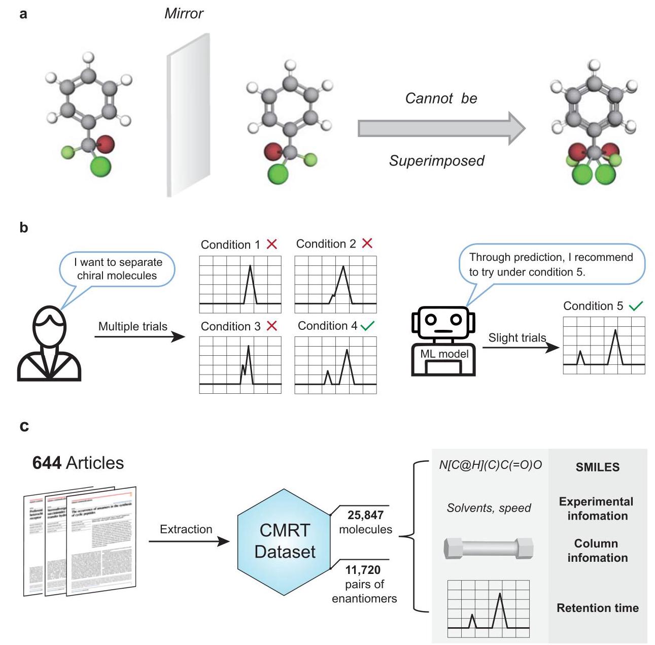
procedure and contents of the chiral molecular retention time dataset (CMRT dataset) in this work. Experimental data of 25,847 molecules (including 11,720 pairs of enantiomers) are extracted from 644 articles about asymmetric catalysis, containing SMILES, experimental information, HPLC column information, and corresponding retention time.

这项工作中手性分子保留时间数据集(CMRT数据集)的过程和内容。从644篇关于不对称催化的文章中提取了25847个分子(包括11720对对映体)的实验数据，其中包含SMILES、实验信息、HPLC柱信息以及相应的保留时间。

Fig. 1 | The scheme for chromatographic enantioseparation. a The diagram for chiral molecules, which are mirror images of each other, but not superimposable. b The comparison between classic separation ways by multiple trials with different conditions and machine learning (ML) models that can recommend the most suitable conditions with the highest separation probability. c The generation

图1 | 色谱对映体分离方案。a手性分子的示意图，它们是彼此的镜像，但不能重叠。b通过不同条件的多次试验进行经典分离方法与能够推荐分离概率最高的最合适条件的机器学习(ML)模型之间的比较。c生成

Nature Communications | (2023)14:3095

《自然·通讯》| (2023)14:3095

the retention time of 25,847 molecules, which contains 11,720 pairs of enantiomers, experimental information, and HPLC column information. The molecules are recorded in the form of SMILES (Fig. 1c).

25,847种分子的保留时间，其中包含11,720对对映体、实验信息和高效液相色谱柱信息。这些分子以SMILES形式记录(图1c)。

2. A machine learning framework called quantile geometry-enhanced graph neural network (QGeoGNN) is constructed by combining quantile learning and GeoGNN, which takes the data uncertainty and chiral molecular representation into consideration and shows satisfactory performance in predicting retention times of chiral molecules. In this framework, the domain knowledge of chromatography and experimental conditions are also incorporated into the model to enhance its extendibility.

3. 一种名为分位数几何增强图神经网络(QGeoGNN)的机器学习框架通过结合分位数学习和GeoGNN构建而成，该框架考虑了数据不确定性和手性分子表示，并在预测手性分子的保留时间方面表现出令人满意的性能。在此框架中，色谱领域知识和实验条件也被纳入模型以增强其可扩展性。

4. The prediction model can guide chromatographic enantiose-paration by predicting the separation possibility in different conditions and thus eliminating repeated trials, which provides a framework for the utilization of machine learning techniques to facilitate experimental chemistry where data are expensive and unstandardized.

5. 该预测模型可以通过预测不同条件下的分离可能性来指导色谱对映体分离，从而消除重复试验，这为利用机器学习技术促进实验化学提供了一个框架，在实验化学中数据昂贵且不规范。

Results

结果

Backgrounds and the CMRT dataset

背景与CMRT数据集

As a ubiquitous phenomenon in nature, molecular chirality is a significant factor that affects molecular properties. A pair of chiral molecules is termed as enantiomers, which are mirror images of each other, but not superimposable (Fig. 1a). Although the molecular constitution of enantiomers is identical with the same atoms and bonds, their properties may be disparate due to the chirality. As an example, left-handed thalidomide is an effective tranquilizer for parturition, while the right-handed enantiomer leads to developmental abnormality in fetuses, and the mixture of enantiomers in the drug once triggered a tragedy ${}^{27}$ . Generally, separating chiral molecules is a challenge because the constitutions of chiral molecules are identical. In order to obtain enantiomerically pure compounds, several chromatographic enantioseparation techniques have been developed in the past decades to separate and analyze the chiral compounds ${}^{28}$ . Among these techniques, high-performance liquid chromatography (HPLC) becomes the mainstream way benefiting from its high efficiency and popularity ${}^{21}$ . In HPLC, the retention time (RT) is a fundamental characteristic, which is defined as the time of chromatographic components from injection to peak (Fig. 1b). It can be used as a qualitative basis for chromatographic enantioseparation since each compound corresponds to a retention time under certain condition. In the chromatographic enantioseparation, the normal-phase HPLC column is adopted where stereoregular chiral polymers are employed as chiral stationary phases (CSPs) to differentiate chiral molecules. Considering that there exist diversified CSPs, different types of HPLC columns have discrepant chiral recognition capacities for different chiral compounds. However, the choice of experimental conditions, including the column type, flow speed, and elution proportion, is currently determined by experience and repeated trials (Fig. 1b). Therefore, this work attempts to construct a machine learning prediction model to predict retention times of chiral molecules and thus facilitating chromatographic enantioseparation.

作为自然界中普遍存在的现象，分子手性是影响分子性质的一个重要因素。一对手性分子被称为对映体，它们是彼此的镜像，但不能重叠(图1a)。尽管对映体的分子组成相同，具有相同的原子和键，但由于手性，它们的性质可能不同。例如，左旋沙利度胺是一种有效的分娩镇静剂，而右旋对映体则会导致胎儿发育异常，该药物中的对映体混合物曾引发一场悲剧${}^{27}$。一般来说，分离手性分子是一项挑战，因为手性分子的组成相同。为了获得对映体纯的化合物，在过去几十年里已经开发了几种色谱对映体分离技术来分离和分析手性化合物${}^{28}$。在这些技术中，高效液相色谱(HPLC)因其高效率和广泛应用而成为主流方法${}^{21}$。在HPLC中，保留时间(RT)是一个基本特征，它被定义为色谱组分从进样到出峰的时间(图1b)。由于每种化合物在特定条件下都对应一个保留时间，因此它可以用作色谱对映体分离的定性依据。在色谱对映体分离中，采用正相HPLC柱，其中立体规整的手性聚合物用作手性固定相(CSP)来区分手性分子。考虑到存在多种CSP，不同类型的HPLC柱对不同的手性化合物具有不同的手性识别能力。然而，目前实验条件的选择，包括柱类型、流速和洗脱比例，是由经验和反复试验决定的(图1b)。因此，这项工作试图构建一个机器学习预测模型来预测手性分子的保留时间，从而促进色谱对映体分离。

To achieve this goal, the CMRT dataset is established by automatically extracting experimental results from the relevant literature, the extraction procedure of which is provided in the Method section. Several interesting aspects of the field of asymmetric catalysis can be reflected in the statistical analysis of the dataset including the contribution of authors, the average new enantiomers reported in the literature, and the usage frequency of HPLC columns, which are detailed in Supplementary Information S1.1. Meanwhile, visualization of molecules in the CMRT dataset is provided in Supplementary Fig. 3.

为了实现这一目标，通过从相关文献中自动提取实验结果建立了CMRT数据集，其提取过程在方法部分提供。数据集的统计分析可以反映不对称催化领域的几个有趣方面，包括作者的贡献、文献中报道的平均新对映体以及HPLC柱的使用频率，这些在补充信息S1.1中有详细说明。同时，补充图3提供了CMRT数据集中分子的可视化。

Construction of QGeoGNN

QGeoGNN的构建

Benefiting from the natural graphic attribute of molecular structure, graph representation has attracted increasing attention in recent years ${}^{29}$ . The atoms and chemical bonds in the molecule are easy to be interpreted as a graph, which is referred to as Graph G (Fig. 2a). The node and edge features in Graph G are related to the characteristics of the molecular atoms and bonds, respectively. Meanwhile, considering that the bond length and angle can reflect the information of 3D conformation, another bond-angle graph, Graph H, is constructed as a complement for Graph G to incorporate geometry characteristics. In Graph H, the node feature is the bond length and the edge feature is the bond angle (Fig. 2a). Compared with traditional molecular representations, the graph representation can reflect chirality by the chiral tags for labeling the handedness of chiral centers. Based on Graph G and H, the quantile geometry-enhanced graph neural network (QGeoGNN) is constructed. As illustrated in Fig. 2b, the proposed QGeoGNN takes experimental settings (i.e., elution proportion) into consideration, which makes the framework more appropriate to address practical experimental scenes. Meanwhile, the incorporation of relevant molecular descriptors further assists to distinguish enantiomers from macroscopic molecular properties. Through the graph convolution, the graph representations are obtained and then transformed into the prediction through a fully-connected layer. Details for the construction of QGeoGNN are provided in the Method section.

得益于分子结构的自然图形属性，图形表示近年来受到越来越多的关注${}^{29}$ 。分子中的原子和化学键很容易被解释为一个图形，称为图G(图2a)。图G中的节点和边特征分别与分子原子和键的特征相关。同时，考虑到键长和键角可以反映三维构象的信息，另一个键角图，图H，被构建为图G的补充，以纳入几何特征。在图H中，节点特征是键长，边特征是键角(图2a)。与传统的分子表示相比，图形表示可以通过标记手性中心手性的手性标签来反映手性。基于图G和H，构建了分位数几何增强图神经网络(QGeoGNN)。如图2b所示，所提出的QGeoGNN考虑了实验设置(即洗脱比例)，这使得该框架更适合于处理实际实验场景。同时，纳入相关的分子描述符有助于从宏观分子性质上区分对映体。通过图卷积，获得图形表示，然后通过全连接层将其转换为预测。QGeoGNN构建的详细信息在方法部分提供。

According to the chromatographic process equation ${}^{30}$ , there exists an inverse proportional relationship between the retention time and flow rate, which is written as:

根据色谱过程方程${}^{30}$ ，保留时间和流速之间存在反比例关系，可写为:

where ${RT}$ is the retention time, $K$ is the partition coefficient, $v$ is the flow rate, ${V}_{m}$ and ${V}_{s}$ are the volume of mobile and stationary phase, ${t}_{O}$ is the dead time, respectively. The equation has been verified through experiments in our laboratory with controlled experimental conditions, as described in the Method section. However, since the data used in this study were collected from diverse literature sources, variations in experimental environments may affect the accuracy of the equation. In general, we expect the overall error of the equation to be around $1(\mathrm{{min}} \times \mathrm{{mL}}/$ min), which is an acceptable level of accuracy for most applications. Upon analysis of the CMRT dataset, we discover that the measured error of the equation is 1.37, which is slightly higher than the expected error but still within an acceptable range (Supplementary Fig. 4). It is important to note that this level of error is not expected to affect the prediction of enantiosepara-tion, as the experimental conditions for enantiomers will be the same. Therefore, the prediction target is set to be ${RT} \times v$ (abbreviated as ${RTv}$ ) in this work to incorporate the chromatographic process equation. Another important component of the proposed QGeoGNN is the utilization of quantile learning, which takes uncertainty into account. Conventional retention time prediction tasks usually focused on the accuracy of the predicted retention time while the uncertainty is neglected. However, the experimental error will bring inevitable deviations to the measured retention time. Specifically, in this case, the task of the prediction model is not only to predict the retention time but also to further guide chromatographic enantioseparation. Traditionally, whether enantiomers can be separated is decided by the difference between retention times, and the threshold is very small (usually tens of seconds), which means the uncertainty and errors have a great influence on whether the enantiomers are predicted to be separable. Therefore, this work adopts an alternative way to involve uncertainty to calculate the separation probability. The measurement of uncertainty in deep learning models has been studied extensively and diversified techniques have been proposed, including the Bayesian techniques ${}^{{31},{32}}$ , probability distribution modeling ${}^{33}$ , and quantile learning ${}^{34}$ . Compared with other methods that require sophisticated modification of the model, quantile learning has better universality and applicability since it can predict the percentiles by simply adding quantile loss to the loss function, which is written as:

其中${RT}$ 是保留时间，$K$ 是分配系数，$v$ 是流速，${V}_{m}$ 和${V}_{s}$ 分别是流动相和固定相的体积，${t}_{O}$ 是死时间。该方程已在我们实验室的受控实验条件下通过实验验证，如方法部分所述。然而，由于本研究中使用的数据是从不同的文献来源收集的，实验环境的变化可能会影响方程的准确性。一般来说，我们期望方程的总体误差在$1(\mathrm{{min}} \times \mathrm{{mL}}/$ 分钟左右，这对于大多数应用来说是一个可接受的精度水平。在分析CMRT数据集时，我们发现该方程的测量误差为1.37，略高于预期误差，但仍在可接受范围内(补充图4)。需要注意的是，这种误差水平预计不会影响对映体分离的预测，因为对映体的实验条件将是相同的。因此，在这项工作中，预测目标被设置为${RT} \times v$ (简称为${RTv}$ )，以纳入色谱过程方程。所提出的QGeoGNN的另一个重要组成部分是分位数学习的应用，它考虑了不确定性。传统的保留时间预测任务通常关注预测保留时间的准确性，而忽略了不确定性。然而，实验误差会给测量的保留时间带来不可避免的偏差。具体来说，在这种情况下，预测模型的任务不仅是预测保留时间，而且还要进一步指导色谱对映体分离。传统上，对映体是否能够分离取决于保留时间之间的差异，并且阈值非常小(通常为几十秒)，这意味着不确定性和误差对对映体是否可预测分离有很大影响。因此，这项工作采用了一种替代方法来纳入不确定性以计算分离概率。深度学习模型中不确定性的测量已经得到了广泛研究，并提出了多种技术，包括贝叶斯技术${}^{{31},{32}}$ 、概率分布建模${}^{33}$ 和分位数学习${}^{34}$ 。与其他需要对模型进行复杂修改的方法相比，分位数学习具有更好的通用性和适用性，因为它可以通过简单地在损失函数中添加分位数损失来预测百分位数，可写为:

(2)

$$

• \mathop{\sum }\limits_{{i = {y}{i}^{\text{ true }} \geq {y}{i}^{\alpha }}}{0.01\alpha }\left| {{y}{i}^{\text{ true }} - {y}{i}^{\alpha }}\right| $$

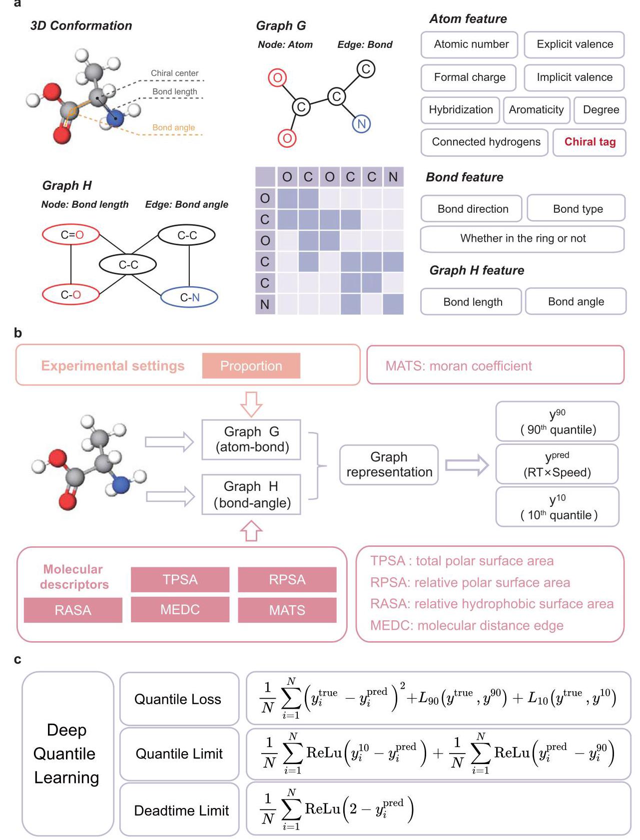
Fig. 2 | The construction of QGeoGNN. a An example of the translation from the 3D conformation of a molecule to two graphs including the atom-bond Graph G and the bond-angle Graph H. Each graph consists of node, edge, and corresponding features. The edges are represented in the form of the adjacent matrix. b The scheme of the QGeoGNN, the experimental settings, and molecular descriptors are incorporated in Graph G and H, respectively. The output neuron of QGeoGNN is 3, namely, the 90th quantile, the prediction, and the 10th quantile. c The constituent of the loss function in QGeoGNN, including the quantile loss, the quantile limit, and the deadtime limit. Here, ${y}^{\text{ true }},{y}^{\text{ pred }},{y}^{10}$ , and ${y}^{90}$ are the observation, prediction, the predicted 10th quantile, and the predicted 90th quantile, respectively. ReLu refers to the linear rectification function.

图2 | QGeoGNN的构建。a一个从分子的3D构象转换为两个图的示例，包括原子-键图G和键角图H。每个图由节点、边和相应的特征组成。边以邻接矩阵的形式表示。b QGeoGNN的方案，实验设置和分子描述符分别纳入图G和H中。QGeoGNN的输出神经元为3个，即第90百分位数、预测值和第10百分位数。c QGeoGNN中损失函数的组成部分，包括分位数损失、分位数限制和死时间限制。这里，${y}^{\text{ true }},{y}^{\text{ pred }},{y}^{10}$和${y}^{90}$分别是观测值、预测值、预测的第10百分位数和预测的第90百分位数。ReLu指线性整流函数。

where ${L}_{\alpha }$ is the quantile loss, $\alpha$ is the quantile, ${y}^{\text{ true }}$ and ${y}^{\alpha }$ are the observed data and the quantile prediction. In this work, the loss function of QGeoGNN consists of three parts, namely quantile loss, quantile limit, and deadtime limit (Fig. 2c). The quantile loss enables the QGeoGNN to learn the predicted value, 90th quantile, and 10th quantile simultaneously, while the quantile limit and deadtime limit function as the constraints to make outputs conform to the mathematical and physical restriction.

其中${L}_{\alpha }$是分位数损失，$\alpha$是分位数，${y}^{\text{ true }}$和${y}^{\alpha }$是观测数据和分位数预测值。在这项工作中，QGeoGNN的损失函数由三部分组成，即分位数损失、分位数限制和死时间限制(图2c)。分位数损失使QGeoGNN能够同时学习预测值、第90百分位数和第10百分位数，而分位数限制和死时间限制起到约束作用，使输出符合数学和物理限制。

Single-column prediction

单柱预测

As illustrated in Fig. 3a, in the area of asymmetric catalysis, various kinds of columns are adopted to handle diversified molecules due to the difficulty of chromatographic enantioseparation. The differences between HPLC column types come from many aspects like CSPs and column model, which affects the chiral recognition ability of HPLC column towards a wide variety of compounds. Among them, ADH, ODH, IC, IA, and OJH are the most frequently utilized column types in the dataset that we collected. From Fig. 3b, it can be seen that the probability density distribution of the retention times in these columns is similar, where the RTs of most molecules are in the range of $5\mathrm{\;{min}}$ to ${30}\mathrm{\;{min}}$ . To better demonstrate the prediction ability of the proposed QGeoGNN, in this section, single-column prediction is conducted where a prediction model is created in each column type. The benefits of the single-column prediction lie in that the conditions of the column are fixed in each predictive model, which means that the data has a good consistency and is conducive to learning the underlying molecule structure-retention time relationship. For each model, the dataset is split into the training dataset, validating dataset, and testing dataset by ${90}/5/5$ . The training dataset is utilized to train the model and the validating dataset is employed for early stopping. The testing data is utilized to examine the model’s performance of the out-of-sample prediction. Considering the distribution of RT values, data points with ${RTv}$ greater than 60 are dropped. The predicted results and corresponding mean average error (MAE), median relative error (MRE), and ${R}^{2}$ are shown in Fig. 3c. It is observed that the QGeoGNN has a good predictive ability for each column with ${R}^{2}$ all larger than 0.7 and the MAE all below 3, which indicates that the molecular structure-retention time relationship has been learned well.

如图3a所示，在不对称催化领域，由于色谱对映体分离的困难，采用了各种类型的色谱柱来处理多样化的分子。高效液相色谱柱类型之间的差异来自多个方面，如手性固定相(CSPs)和色谱柱模型，这影响了高效液相色谱柱对多种化合物的手性识别能力。其中，ADH、ODH、IC、IA和OJH是我们收集的数据集中最常用的色谱柱类型。从图3b可以看出，这些色谱柱中保留时间的概率密度分布相似，其中大多数分子的保留时间在$5\mathrm{\;{min}}$到${30}\mathrm{\;{min}}$范围内。为了更好地展示所提出的分位数几何增强图神经网络(QGeoGNN)的预测能力，在本节中进行单柱预测，即在每种色谱柱类型中创建一个预测模型。单柱预测的好处在于，在每个预测模型中色谱柱的条件是固定的，这意味着数据具有良好的一致性，有利于学习潜在的分子结构-保留时间关系。对于每个模型，数据集通过${90}/5/5$分为训练数据集、验证数据集和测试数据集。训练数据集用于训练模型，验证数据集用于提前停止。测试数据用于检验模型的样本外预测性能。考虑到保留时间(RT)值的分布，删除了${RTv}$大于60的数据点。预测结果以及相应的平均绝对误差(MAE)、中位数相对误差(MRE)和${R}^{2}$如图3c所示。可以观察到，QGeoGNN对每根色谱柱都具有良好的预测能力，${R}^{2}$均大于0.7，MAE均低于3，这表明分子结构-保留时间关系已被很好地学习。

To eliminate the influence of randomness in splitting the dataset, cross-validation is conducted for each column type, and the results are shown in Supplementary Fig. 5. From cross-validation, it is discovered that the model’s performance is restricted to some extent since there exist multiple mild outliers, which means the prediction accuracy of the model for some samples needs to be improved. As intuitively discovered in the previous literature ${}^{25}$ , the performance of the ML model usually depends on the similarity between the predicted and trained molecule’s structure. Considering that the advantage of using the ML model instead of just using literature search for retention time prediction and chromatographic enantioseparation is to be able to predict the enantiomers not reported in the literature, the generalization ability of the model to enantiomers with different levels of similarity is further investigated. In this study, the Tanimoto similarity coefficient is employed to measure the similarity between 2D structures of two molecules, the range of which is from 0% to 100%. For each model in cross-validation, the Tanimoto similarity coefficient between each enantiomer in the testing dataset and all enantiomers in the training dataset are calculated. Several similarity thresholds are utilized to differentiate the similarity level including 95%, 90%, 80%, 70%, 60%, and 50%. Therefore, all data are categorized into six groups where the molecules in each group as the testing dataset have at least one similar molecule in the training dataset above a specific similarity threshold. The ODH model is taken as an example here, where the size of groups are ${n}_{95} = {923}\left( {{18.7}\% }\right) ,{n}_{90} = {1009}\left( {{20.4}\% }\right) ,{n}_{80} = {1672}\left( {{33.8}\% }\right)$ , ${n}_{70} = {3030}\left( {{61.3}\% }\right) ,\;{n}_{60} = {3956}\left( {{80.1}\% }\right)$ , and ${n}_{50} = {4491}\left( {{90.9}\% }\right)$ , respectively. Of note, there are 9.1% of enantiomers whose similarity with any molecule in the training dataset do not exceed 50%. The MAE and MRE of the prediction in these groups are illustrated in Fig. 3d. It is confirmed that the generalization ability is highly related to the molecular similarity since the prediction accuracy of the model diminishes evidently with the decrease of similarity. For molecules with over 90% similarity, the model’s performance is satisfactory with average relative and absolute errors of only 12.7% and 2.0, while the error raises to 15.7% and 3.0 with over 50% similarity. Compared with existing literature that predicts retention time in UPLC ${}^{35}$ and reversed-phase HPLC ${}^{25}$ , the prediction error of our model is slightly higher. It is mainly because the inner similarity of the CMRT dataset obtained from the literature is overall lower than the dataset obtained from actual experiments. Meanwhile, the task of chromatographic enantiose-paration in normal-phase HPLC is more complex and the retention times are typically longer.

为消除数据集划分中随机性的影响，对每种色谱柱类型进行了交叉验证，结果见补充图5。通过交叉验证发现，由于存在多个轻度异常值，模型的性能在一定程度上受到限制，这意味着模型对某些样品的预测准确性有待提高。正如之前文献${}^{25}$中直观发现的那样，机器学习模型的性能通常取决于预测分子与训练分子结构之间的相似性。考虑到使用机器学习模型而非仅通过文献检索进行保留时间预测和色谱对映体分离的优势在于能够预测文献中未报道的对映体，因此进一步研究了模型对不同相似性水平对映体的泛化能力。在本研究中，采用Tanimoto相似系数来衡量两个分子二维结构之间的相似性，其范围为0%至100%。对于交叉验证中的每个模型，计算测试数据集中每个对映体与训练数据集中所有对映体之间的Tanimoto相似系数。利用几个相似性阈值来区分相似性水平，包括95%、90%、80%、70%、60%和50%。因此，所有数据被分为六组，其中每组作为测试数据集的分子在训练数据集中至少有一个相似分子高于特定的相似性阈值。这里以ODH模型为例，其中各组的大小分别为${n}_{95} = {923}\left( {{18.7}\% }\right) ,{n}_{90} = {1009}\left( {{20.4}\% }\right) ,{n}_{80} = {1672}\left( {{33.8}\% }\right)$、${n}_{70} = {3030}\left( {{61.3}\% }\right) ,\;{n}_{60} = {3956}\left( {{80.1}\% }\right)$和${n}_{50} = {4491}\left( {{90.9}\% }\right)$。值得注意的是，有9.1%的对映体与训练数据集中任何分子的相似性不超过50%。这些组中预测的平均绝对误差(MAE)和平均相对误差(MRE)如图3d所示。可以确认，泛化能力与分子相似性高度相关，因为模型的预测准确性随着相似性的降低而明显下降。对于相似性超过90%的分子，模型的性能令人满意，平均相对误差和绝对误差仅为12.7%和2.0，而相似性超过50%时误差升至15.7%和3.0。与预测超高效液相色谱(UPLC)${}^{35}$和反相高效液相色谱(HPLC)${}^{25}$中保留时间的现有文献相比，我们模型的预测误差略高。这主要是因为从文献中获得的CMRT数据集的内部相似性总体低于从实际实验中获得的数据集。同时，正相高效液相色谱中的色谱对映体分离任务更为复杂，保留时间通常更长。

To better reveal the predictive ability of the proposed QGeoGNN, the influence of data volume and noise is investigated where the prediction on the ODH column is taken as an example. The data noise is added as:

为了更好地揭示所提出的QGeoGNN的预测能力，以ODH柱上的预测为例，研究了数据量和噪声的影响。添加的数据噪声如下:

where $\widehat{y}$ is the noisy data, $y$ is the observation data, ${std}\left( y\right)$ refers to the standard deviation of the observation data, and $N\left( {0,1}\right)$ is the normal distribution. The results are illustrated in Fig. 3d. It is discovered that the QGeoGNN is robust to data noise since the performance maintains stability faced with 10% data noise. At the same time, the observation data itself has inevitable experimental errors, which further verifies the superiority of the proposed method in dealing with noise. In terms of data volume, it is found that the prediction accuracy increases with the increase of training data ratio, and the trend of increase keeps apparent with 90% of the data, which means that if more sufficient data is provided, the prediction accuracy of QGeoGNN still has ample room for improvement.

其中$\widehat{y}$是噪声数据，$y$是观测数据，${std}\left( y\right)$是观测数据的标准差，$N\left( {0,1}\right)$是正态分布。结果如图3d所示。发现QGeoGNN对数据噪声具有鲁棒性，因为面对10%的数据噪声时性能保持稳定。同时，观测数据本身存在不可避免的实验误差，这进一步验证了所提出方法在处理噪声方面的优越性。在数据量方面，发现预测准确性随着训练数据比例的增加而提高，并且在90%的数据时增加趋势仍然明显，这意味着如果提供更充分的数据，QGeoGNN的预测准确性仍有很大的提升空间。

Multi-column prediction

多柱预测

On the basis of the satisfactory performance of QGeoGNN in single-column prediction which confirms that the proposed framework is able to learn the molecular structure-retention relationship well, multi-column prediction is conducted in this section that acquires to integrate the prediction of diversified types of columns into a synthetic model. Here, the domain knowledge of chromatography is combined with machine learning techniques to facilitate model construction. In the HPLC column that is depicted in Fig. 4a, CSPs are derived from polysaccharides, including cellulose and amylose which are some of the most common chiral bio-based polymers in nature. As the insufficient chiral recognition ability of cellulose and amylose, their derivatives such as esters and carbamates modified with corresponding substituents are more frequently applied for both analytical and preparative enantioseparations ${}^{36}$ . The CSPs are usually immobilized or coated to silica gel. Therefore, in this work, three main factors are taken into consideration that affect the chiral recognition performance of HPLC columns, including the CSPs, the connection type (immobilized or coated), and the packing material (silica) size.

基于QGeoGNN在单柱预测中的良好性能，这证实了所提出的框架能够很好地学习分子结构 - 保留关系，在本节中进行多柱预测，旨在将多种类型柱的预测整合到一个综合模型中。在这里，色谱领域知识与机器学习技术相结合以促进模型构建。在图4a所示的HPLC柱中，手性固定相(CSPs)衍生自多糖，包括纤维素和直链淀粉，它们是自然界中一些最常见的基于生物的手性聚合物。由于纤维素和直链淀粉的手性识别能力不足，它们的衍生物，如用相应取代基修饰的酯和氨基甲酸酯，更常用于分析和制备对映体分离${}^{36}$。CSPs通常固定或涂覆在硅胶上。因此，在这项工作中，考虑了影响HPLC柱手性识别性能的三个主要因素，包括CSPs、连接类型(固定或涂覆)和填充材料(硅胶)尺寸。

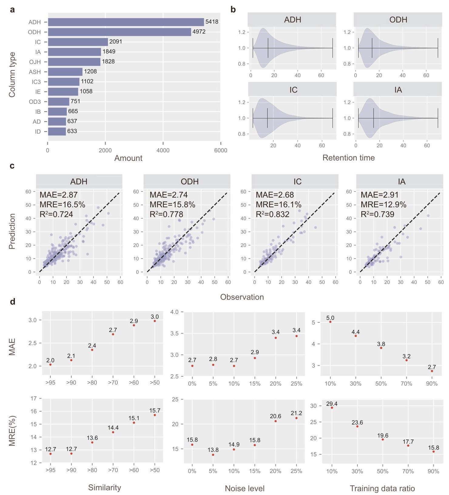
Fig. 3 | The performance of QGeoGNN for single-column prediction. a The data amount of each column type in the CMRT dataset established in this work. Only the first 12 column types with the largest volume are displayed here. $\mathbf{b}$ The violin plot of the retention time in the subset of ADH (5418 data), ODH (4972 data), IC (2091 data), and IA columns (1849 data). The black lines mean the minimum, median, and maximum values, respectively. Molecules with retention time larger than 70 min are rare and are regarded as outliers. c Observation versus prediction for the proposed QGeoGNN to predict out-of-sample molecules. Only testing data are shown in plots. The dashed line is the $y = x$ line. The measurements are the mean average error (MAE), median relative error (MRE), and coefficient of determination $\left( {R}^{2}\right) .\mathbf{d}$ The influence of similarity (left), data noise (middle), and data volume (right) on the single-column prediction model. Source data are provided as a Source Data file.

图3 | QGeoGNN用于单柱预测的性能。a 本工作中建立的CMRT数据集中每种柱类型的数据量。这里仅显示体积最大的前12种柱类型。$\mathbf{b}$ ADH(5418个数据)、ODH(4972个数据)、IC(2091个数据)和IA柱(1849个数据)子集中保留时间的小提琴图。黑线分别表示最小值、中位数和最大值。保留时间大于70分钟的分子很少，被视为异常值。c 所提出的QGeoGNN预测样本外分子的观测值与预测值。图中仅显示测试数据。虚线是$y = x$线。测量值是平均绝对误差(MAE)、中位数相对误差(MRE)和决定系数$\left( {R}^{2}\right) .\mathbf{d}$ 相似性(左)、数据噪声(中)和数据量(右)对单柱预测模型的影响。源数据作为源数据文件提供。

In this work, all types of HPLC columns in the dataset are composed of different collocations of two substrates and seven sub-stituents (Fig. 4a). The substrate is digitized by 0 (amylose) and 1 (cellulose), and the connection type is digitized similarly by 0 (immobilized) and 1 (coated). They are incorporated into the edge features in Graph G of QGeoGNN along with the packing material size (Fig. 4b). The properties of CSPs described by relevant descriptors are added to the edge features in Graph H. As illustrated in Fig. 4b, the edge features of Graph G and Graph H can be represented by feature matrixes and the incorporation of column features can be conducted by the augmentation of the respective feature matrix. Details of the incorporation of column information are provided in the Method section. In this way, all data in the CMRT dataset can be adapted to train a synthetic model for multi-column prediction, which enhances the availability of data. Considering that it is unrealistic to establish single-column prediction models for some less frequently used columns, where the data volume is small and insufficient for model construction, the multi-column prediction models combine the domain knowledge of chromatography with the machine learning model so that it can handle a variety of columns, which further improves the flexibility and scalability of the framework. The predictive performance of the multi-column prediction models is illustrated in Fig. 5a, where the entire data is split into ${90}/5/5$ and the prediction on testing data is depicted in the figure. Faced with data from diversified columns and experimental conditions, the ${R}^{2}$ and MAE of the predictive model still achieve 0.702 and 3.40, which confirms the predictive ability of the synthetic model. An additional experiment is conducted in Supplementary Information S2.3 to observe the influence of column features in the multi-column prediction, and the results show that the incorporation of column information is of great importance for the accuracy of QGeoGNN.

在这项工作中，数据集中的所有类型HPLC柱由两种底物和七种取代基的不同搭配组成(图4a)。底物用0(直链淀粉)和1(纤维素)数字化，连接类型同样用0(固定)和1(涂覆)数字化。它们与填充材料尺寸一起被纳入QGeoGNN的图G的边特征中(图4b)。由相关描述符描述的CSPs的属性被添加到图H的边特征中。如图4b所示，图G和图H的边特征可以由特征矩阵表示，并且柱特征的合并可以通过相应特征矩阵的扩充来进行。柱信息合并的详细内容在方法部分提供。通过这种方式，CMRT数据集中的所有数据都可以用于训练多柱预测的综合模型，这提高了数据的可用性。考虑到为一些使用频率较低的柱建立单柱预测模型是不现实的，因为其数据量小且不足以构建模型，多柱预测模型将色谱领域知识与机器学习模型相结合，以便能够处理各种柱，这进一步提高了框架的灵活性和可扩展性。多柱预测模型的预测性能在图5a中示出，其中整个数据被拆分为${90}/5/5$，并且图中描绘了对测试数据的预测。面对来自多种柱和实验条件的数据，预测模型的${R}^{2}$和MAE仍然达到0.702和3.40，这证实了综合模型的预测能力。在补充信息S2.3中进行了一项额外实验以观察多柱预测中柱特征的影响，结果表明柱信息的合并对QGeoGNN的准确性非常重要。

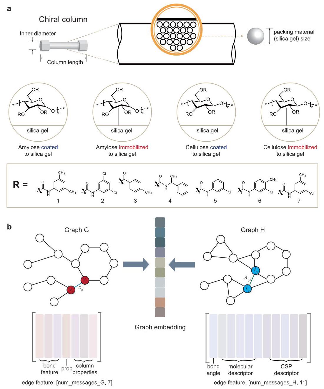
Fig. 4 | The incorporation of column features in multi-column prediction. a The domain knowledge of chromatography by HPLC, which is consisted of the chiral stationary phase (CSP) and mobile phase. For CSPs, the packing material size, substrates, substituents, and connection type (immobilized or coated) will affect the chiral recognition ability of HPLC columns. The inner diameter and column length can also influence the chiral recognition ability, but they are kept the same in commercial HPLC columns. b The illustration for the incorporation of column information. num_messages_G and num_messages_H refer to the number of message paths (normally equals the number of edges) for Graph G and H, respectively. The column properties include the packing material size, substrates (cellulose or amylose), and connection type (immobilized or coated). The CSP descriptor includes moran coefficient (MATS), total polar surface area (TPSA), relative polar surface area (RPSA), relative hydrophobic surface area (RASA), and molecular distance edge (MEDC) of the CSP.

图4 | 多柱预测中柱特征的纳入。a 高效液相色谱(HPLC)的色谱领域知识，由手性固定相(CSP)和流动相组成。对于CSP，填充材料尺寸、底物、取代基和连接类型(固定或涂覆)会影响HPLC柱的手性识别能力。内径和柱长也会影响手性识别能力，但在商用HPLC柱中它们保持不变。b 柱信息纳入的示意图。num_messages_G和num_messages_H分别指图G和图H的消息路径数量(通常等于边的数量)。柱属性包括填充材料尺寸、底物(纤维素或直链淀粉)和连接类型(固定或涂覆)。CSP描述符包括CSP的莫兰系数(MATS)、总极性表面积(TPSA)、相对极性表面积(RPSA)、相对疏水表面积(RASA)和分子距离边(MEDC)。

In order to better demonstrate the superiority of the proposed QGeoGNN, conventional machine learning techniques, including LGB, XGB, artificial neural network (ANN), and GNN, are adopted to train prediction models for comparison. In LGB, XGB, and ANN, the molecular fingerprints and descriptors are employed for representation, while GNN only utilizes Graph G for molecular representation. The column information is incorporated into these models as well and other conditions are kept the same. For LGB, XGB, and ANN, the column information is combined with the input fingerprints and descriptors. For GNN, the column information is formed similarly and incorporated in Graph G. More details of implements of these conventional models are provided in the Method section. The results are provided in Fig. 5b. It is obvious that classic tree-based models like LGB and XGB have poor predictive performance. On the other hand, the ANN can grasp the general relationship, but the accuracy needs to be improved. In comparison, the GNN-based models show superior ability where ${R}^{2}$ of GNN and QGeoGNN achieve 0.620 and 0.702 while the MAE reaches 3.95 and 3.40, respectively. This is an interesting phenomenon since the conventional tree-based and ANN-based models often perform well in most chemical molecular prediction tasks, including previous literature on RT prediction ${}^{{24} - {26}}$ . In order to reveal the reasons behind this phenomenon explicitly, we provide the prediction of two pairs of example enantiomers given by different machine learning models in Table 1. It is evident that the conventional models have difficulty in differentiating enantiomers since the predicted RTs are very close, even the same, which accounts for the poor performance on the CMRT dataset with enantiomers. In contrast, the QGeoGNN can not only distinguish enantiomers well but also provide an accurate predicted RT and its value range. The results demonstrate that the representation of chiral information is of great significance in the chromatographic enantioseparation task considered in this work, and the graph is proven to be a superior representation method than the conventional molecular fingerprints and descriptors when dealing with enantiomers. In addition, compared with GNN, the additional Graph H that incorporates the information of 3D conformation assists to learn the inherent molecular structure-retention relationship, which further improves the predictive ability of the model.

为了更好地证明所提出的QGeoGNN的优越性，采用包括LightGBM(LGB)、XGBoost(XGB)、人工神经网络(ANN)和图神经网络(GNN)在内的传统机器学习技术来训练预测模型进行比较。在LGB、XGB和ANN中，分子指纹和描述符用于表示，而GNN仅利用图G进行分子表示。柱信息也被纳入这些模型，其他条件保持相同。对于LGB、XGB和ANN，柱信息与输入的指纹和描述符相结合。对于GNN，柱信息以类似方式形成并纳入图G。这些传统模型的实现细节在方法部分提供。结果在图5b中给出。很明显，像LGB和XGB这样的经典基于树的模型预测性能较差。另一方面，ANN可以掌握一般关系，但准确性需要提高。相比之下，基于GNN的模型表现出优越的能力，其中GNN和QGeoGNN的${R}^{2}$分别达到0.620和0.702，而平均绝对误差(MAE)分别达到3.95和3.40。这是一个有趣的现象，因为传统的基于树的和基于ANN的模型在大多数化学分子预测任务中通常表现良好，包括之前关于保留时间预测的文献${}^{{24} - {26}}$ 。为了明确揭示这一现象背后的原因，我们在表1中提供了不同机器学习模型给出的两对示例对映体的预测。很明显，传统模型难以区分对映体，因为预测的保留时间非常接近，甚至相同，这导致在含有对映体的CMRT数据集中性能较差。相比之下，QGeoGNN不仅可以很好地区分对映体，还可以提供准确的预测保留时间及其值范围。结果表明，手性信息的表示在本工作中考虑的色谱对映体分离任务中具有重要意义，并且在处理对映体时，图被证明是一种比传统分子指纹和描述符更优越的表示方法。此外，与GNN相比，纳入3D构象信息的附加图H有助于学习固有的分子结构 - 保留关系，这进一步提高了模型的预测能力。

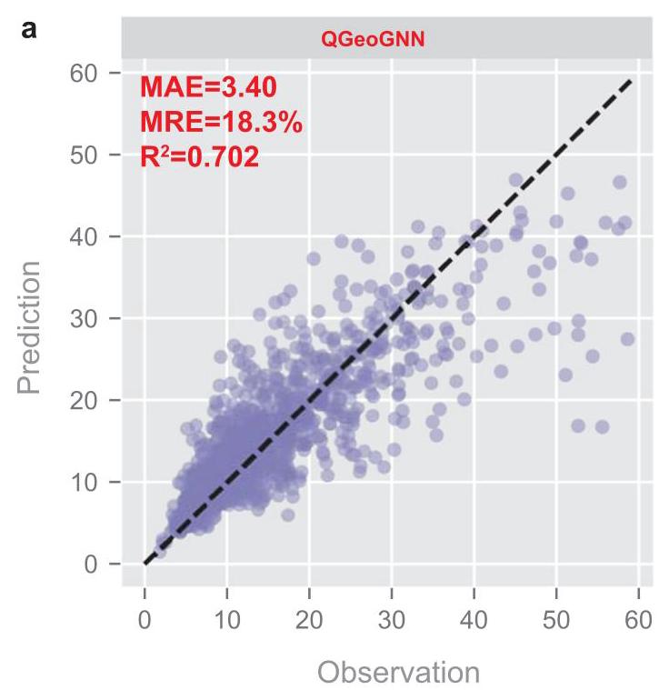
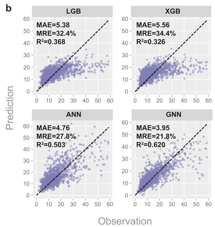
Fig. 5 | The comparison between QGeoGNN and conventional machine learning techniques for multi-column prediction. a Observation versus prediction for the proposed QGeoGNN to predict out-of-sample molecules in diversified high-performance liquid chromatography (HPLC) columns. b Observation versus prediction for LightGBM (LGB), XGBoost (XGB), artificial neural network (ANN), and graph neural network (GNN) for comparison. Only testing data are shown in plots. The dashed line is the $y = x$ line. The measurements are the mean average error (MAE), median relative error (MRE), and coefficient of determination $\left( {R}^{2}\right)$ . Source data are provided as a Source Data file.

图5 | QGeoGNN与传统机器学习技术在多柱预测方面的比较。a 所提出的QGeoGNN对多种高效液相色谱(HPLC)柱中的样本外分子进行预测时的观测值与预测值。b LightGBM(LGB)、XGBoost(XGB)、人工神经网络(ANN)和图神经网络(GNN)用于比较的观测值与预测值。图中仅显示测试数据。虚线是$y = x$线。测量指标是平均绝对误差(MAE)、中位数相对误差(MRE)和决定系数$\left( {R}^{2}\right)$ 。源数据作为源数据文件提供。

Chromatographic enantioseparation probability assessment

色谱对映体分离概率评估

The ultimate goal of the retention time prediction model is facilitating chromatographic enantioseparation, which has been an outstanding issue all along. The difficulties for machine learning mainly concentrate on two aspects including chiral representation and error sensitivity. Specifically, chiral representation decides the ability to distinguish enantiomers while the error sensitivity determines the accuracy. Benefiting from the geometry-enhanced graph representation and the quantile learning, the proposed QGeoGNN provides a promising way to handle the above-mentioned challenges and thus facilitate chromatographic enantioseparation. In order to quantitatively evaluate the probability of enantioseparation under certain experimental conditions like column types, flow rate, and elution proportion, a chromatographic separation probability ${S}_{p}$ is proposed based on the predicted value ranges of enantiomers. In this work, ${S}_{p}$ is defined based on the naïve principle that the area within the overlapping part of the value range is considered inseparable, while other areas are separable. The conceptual formula can be written as:

保留时间预测模型的最终目标是促进色谱对映体分离，这一直是一个突出的问题。机器学习的困难主要集中在两个方面，包括手性表示和误差敏感性。具体来说，手性表示决定了区分对映体的能力，而误差敏感性决定了准确性。受益于几何增强图表示和分位数学习，所提出的QGeoGNN为应对上述挑战提供了一种有前途的方法，从而促进色谱对映体分离。为了定量评估在某些实验条件(如柱类型、流速和洗脱比例)下对映体分离的概率，基于对映体的预测值范围提出了一种色谱分离概率${S}_{p}$。在这项工作中，${S}_{p}$是基于一个简单的原则定义的，即值范围重叠部分内的区域被认为是不可分离的，而其他区域是可分离的。概念公式可以写成:

where ${L}_{\text{ separable }}$ refers to the length of the value range in which the enantiomers are predicted to be separable and ${L}_{\text{ total }}$ refers to the total length of the value range. As detailed in the Method section, the separation probability ${S}_{p}$ is derived and calculated as:

其中${L}_{\text{ separable }}$指预测对映体可分离的值范围的长度，${L}_{\text{ total }}$指值范围的总长度。如方法部分所述，分离概率${S}_{p}$的推导和计算如下:

where $R{T}_{90}^{\max }$ and $R{T}_{90}^{\min }$ are the maximum and minimum of 90th percentiles for both enantiomers, $R{T}_{10}^{\max }$ and $R{T}_{10}^{\min }$ are the maximum and minimum of 10th percentiles, respectively (Fig. 6a). The unit of ${RT}$ is minute while ${S}_{p}$ is dimensionless. The defined chromatographic separation probability ${S}_{p}$ ranges from 0 to 1 . A higher ${S}_{p}$ refers to a higher possibility that the enantiomers are predicted to be separable by the model. Some examples are given in Fig. 6a to better illustrate the separation probability. It is found that the proposition of ${S}_{p}$ assists to eliminate the impact of prediction errors to some extent. Specifically, single predicted values have low fault tolerance since the separation threshold is rigorous (usually tens of seconds). In comparison, quantile learning provides potential value ranges in consideration of uncertainty, which can provide a separation probability instead of simple yes or no, which improves fault tolerance rate, and is more meaningful for chromatographic separation. Meanwhile, chromatographic enantioseparation prediction requires the model to learn the difference between enantiomers well. It means that although the prediction error in multi-column prediction (MRE = 18.3%) seems to be much greater than the separation threshold, chromatographic enantioseparation prediction is still possible.

其中$R{T}_{90}^{\max }$和$R{T}_{90}^{\min }$分别是两种对映体第90百分位数的最大值和最小值，$R{T}_{10}^{\max }$和$R{T}_{10}^{\min }$分别是第10百分位数的最大值和最小值(图6a)。${RT}$的单位是分钟，而${S}_{p}$是无量纲的。定义的色谱分离概率${S}_{p}$的范围是0到1。${S}_{p}$越高，表明模型预测对映体可分离的可能性越高。图6a给出了一些例子以更好地说明分离概率。发现${S}_{p}$的提出在一定程度上有助于消除预测误差的影响。具体来说，由于分离阈值很严格(通常为几十秒)，单个预测值的容错性较低。相比之下，分位数学习考虑了不确定性提供了潜在的值范围，它可以提供一个分离概率而不是简单的是或否，这提高了容错率，并且对色谱分离更有意义。同时，色谱对映体分离预测要求模型很好地学习对映体之间的差异。这意味着尽管多柱预测中的预测误差(MRE = 18.3%)似乎远大于分离阈值，但色谱对映体分离预测仍然是可能的。

Table 1 | Predicted retention time of two pairs of example enantiomers given by different machine learning models, including LightGBM (LGB), XGBoost (XGB), artificial neural network (ANN), and the proposed QGeoGNN

表1 | 不同机器学习模型给出的两对示例对映体的预测保留时间，包括LightGBM(LGB)、XGBoost(XGB)、人工神经网络(ANN)以及所提出的QGeoGNN

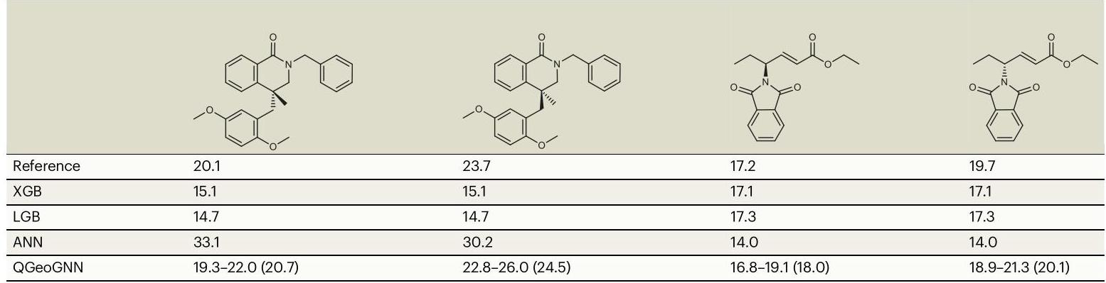
The result of QGeoGNN is presented in the form of the 10th quantile to 90th quantile (predicted retention time)

QGeoGNN的结果以第10百分位数到第90百分位数(预测保留时间)的形式呈现

In order to demonstrate the ability of the proposed model to facilitate chromatographic enantioseparation, several experiments are conducted in this section. First, 412 pairs of enantiomers (i.e., 824 data) are randomly selected from the CMRT dataset to form the testing dataset while the training dataset (23,020 data) and validating dataset (904 data) are randomly chosen from the remaining data to train the prediction model. The separation probability ${S}_{p}$ of the enantiomers in the testing dataset is calculated and illustrated in Fig. 6b. Considering that the proposed separation probability is a naïve estimation of the probability of enantioseparation under certain experimental conditions, the threshold to determine whether enantiomers are regarded as separable is decided in the practical scene to be 0.38 , which is detailed in Supplementary Information S2.4. Therefore, in this work, we regard those enantiomers with ${S}_{p} > {0.38}$ as separable, and the accuracy for the separation of 412 pairs of enantiomers reaches 85.7%. The high accuracy confirms the ability of the proposed QGeoGNN to predict chromatographic enantioseparation. In order to assess the influence of molecular similarity on the accuracy of enantioseparation prediction, additional investigations are conducted using the same methodology as described above. Specifically, we use six similarity thresholds (>95%, >90%, >80%, >70%, >60%, and >50%) to group the molecules, resulting in different group sizes: ${n}_{95} = 4\left( {{0.97}\% }\right) ,{n}_{90} = {17}\left( {{4.13}\% }\right) ,{n}_{80} = {118} \; \left( {{28.6}\% }\right) ,{n}_{70} = {273}\left( {{66.3}\% }\right) ,{n}_{60} = {367}\left( {{89.1}\% }\right)$ , and ${n}_{50} = {403}\left( {{97.8}\% }\right)$ , respectively. As illustrated in Fig. 6c, our results demonstrate that the accuracy of the model is highly dependent on the structural similarity of the enantiomers being predicted. Specifically, the prediction accuracy of the model reaches an accuracy rate of 100% and 94.1% for molecules with a similarity of >95% and >90%, respectively. However, as the similarity threshold decreases, the prediction accuracy of the model also decreases, indicating that the model may have limitations in accurately predicting enantioseparation for more dissimilar compounds. It is worth noting that chromatographic enantioseparation prediction differs from typical classification tasks owing to its distinctive requirements. Considering the difficulty of chromatographic enantioseparation, a suitable separation condition is very important but scarce, which means that it is unaffordable to predict a separable situation as inseparable (Type I error) since it may miss the precious suitable separative conditions. In contrast, it is relatively acceptable to predict the inseparable condition as separable (Type II error), because this will only induce additional experiments. Benefiting from the multi-column prediction accomplished by QGeoGNN, the separation probabilities of the same enantiomers in different types of HPLC columns can be obtained and compared, which can directly reflect the predicted chiral recognition ability of each column to the given enantio-mers, thus providing suggestions on selecting proper experimental conditions without tedious trails and errors. In Fig. 6d, we provide an example of the utilization in practical application. To separate enan-tiomers, multiple candidate conditions composed of six column types and corresponding proportions and flow rates are considered to select the most proper separative condition. The selected column types are those frequently utilized in chromatographic enantioseparation and commonly seen in the organic laboratory. For each column, the proportion and flow rates of the candidate condition are determined by a domain expert that is likely to generate a suitable retention time. If experiments are conducted to try with all these conditions, it will take several hours. In contrast, the QGeoGNN only needs seconds to predict the separation probability under each condition, which can be visually depicted in the figure, and easy to find the most proper situations with the largest ${S}_{p}$ and moderate predicted retention time, thus saving appreciable time for experimenters. The experimental experiments confirm that the enantiomers can only be separated in the IG column, which is consistent with the prediction. For comparison, four conventional techniques including XGB, LGB, ANN, and GNN, are trained under the same condition and tested with the same enantiomer and candidate conditions. The $\bigtriangleup {RT}$ is calculated for each of the candidate conditions, which is denoted as $\left| {R{T}_{1} - R{T}_{2}}\right|$ . The results are depicted in Fig. 6e. Traditionally, whether the enantiomers can be separated is decided by the $\bigtriangleup {RT}$ , and the separation threshold is usually ${0.3}\mathrm{\;{min}}$ (black dotted line in Fig. 6e). It can be seen that ANN, LGB, and XGB cannot distinguish enantiomers since the predicted retention time of enantiomers is similar and even the same ( $\bigtriangleup {RT}$ close to 0). Therefore, these three methods tend to predict all enantiomers to be inseparable, which proves that they do not have the ability for chromatographic enantioseparation prediction. It is found that GNN can learn the difference between enantiomers, however, the prediction is completely wrong. As shown in the figure, it predicts ADH, IC, and ID to be separable while ODH, IG, and ASH are inseparable. Nevertheless, the real situation is that only the IG column can separate the enan-tiomers. It proves the accuracy of GNN is limited and insufficient to provide correct guidance for practical experiments. The comparison further proves the superiority of the proposed QGeoGNN and separation probability in chromatographic enantioseparation prediction.

为了证明所提出模型促进色谱对映体分离的能力，本节进行了几个实验。首先，从CMRT数据集中随机选择412对对映体(即824个数据)形成测试数据集，而训练数据集(23,020个数据)和验证数据集(904个数据)从其余数据中随机选择以训练预测模型。计算测试数据集中对映体的分离概率${S}_{p}$并在图6b中示出。考虑到所提出的分离概率是在某些实验条件下对映体分离概率的简单估计，在实际场景中确定对映体是否可分离的阈值为0.38，这在补充信息S2.4中有详细说明。因此，在本工作中，我们将那些具有${S}_{p} > {0.38}$的对映体视为可分离的，并且412对对映体的分离准确率达到85.7%。高准确率证实了所提出的QGeoGNN预测色谱对映体分离的能力。为了评估分子相似性对对映体分离预测准确性的影响，使用与上述相同的方法进行了额外的研究。具体而言，我们使用六个相似性阈值(>95%、>90%、>80%、>70%、>60%和>50%)对分子进行分组，得到不同的组大小:${n}_{95} = 4\left( {{0.97}\% }\right) ,{n}_{90} = {17}\left( {{4.13}\% }\right) ,{n}_{80} = {118} \; \left( {{28.6}\% }\right) ,{n}_{70} = {273}\left( {{66.3}\% }\right) ,{n}_{60} = {367}\left( {{89.1}\% }\right)$和${n}_{50} = {403}\left( {{97.8}\% }\right)$。如图6c所示，我们的结果表明模型的准确性高度依赖于所预测对映体的结构相似性。具体而言，对于相似度>95%和>90%的分子，模型的预测准确率分别达到100%和94.1%。然而，随着相似性阈值的降低，模型的预测准确率也会降低，这表明该模型在准确预测更不相似化合物的对映体分离方面可能存在局限性。值得注意的是，色谱对映体分离预测由于其独特的要求与典型的分类任务不同。考虑到色谱对映体分离的难度，合适的分离条件非常重要但很少见，这意味着将可分离情况预测为不可分离(I型错误)是不可接受的，因为这可能会错过宝贵的合适分离条件。相比之下，将不可分离条件预测为可分离(II型错误)相对可以接受，因为这只会导致额外的实验。受益于QGeoGNN完成的多柱预测，可以获得并比较同一对映体在不同类型HPLC柱中的分离概率，这可以直接反映每个柱对给定对映体的预测手性识别能力，从而在无需繁琐试验和错误的情况下为选择合适的实验条件提供建议。在图6d中，我们提供了一个实际应用中的示例。为了分离对映体，考虑由六种柱类型以及相应比例和流速组成的多个候选条件，以选择最合适的分离条件。所选的柱类型是在色谱对映体分离中经常使用且在有机实验室中常见的那些。对于每个柱，候选条件的比例和流速由可能产生合适保留时间的领域专家确定。如果对所有这些条件进行实验尝试，则需要数小时。相比之下，QGeoGNN仅需几秒钟即可预测每个条件下的分离概率，这可以在图中直观地描绘出来，并且很容易找到具有最大${S}_{p}$和适中预测保留时间的最合适情况，从而为实验人员节省大量时间。实验证实对映体仅在IG柱中可分离，这与预测一致。作为比较，在相同条件下训练包括XGB、LGB、ANN和GNN在内的四种传统技术，并使用相同的对映体和候选条件进行测试。为每个候选条件计算$\bigtriangleup {RT}$，其表示为$\left| {R{T}_{1} - R{T}_{2}}\right|$。结果如图6e所示。传统上，对映体是否可分离由$\bigtriangleup {RT}$决定，并且分离阈值通常为${0.3}\mathrm{\;{min}}$(图6e中的黑色虚线)。可以看出，ANN、LGB和XGB无法区分对映体，因为对映体的预测保留时间相似甚至相同($\bigtriangleup {RT}$接近0)。因此，这三种方法倾向于预测所有对映体不可分离，这证明它们不具有色谱对映体分离预测的能力。发现GNN可以学习对映体之间的差异，然而，预测完全错误。如图所示，它预测ADH、IC和ID可分离，而ODH、IG和ASH不可分离。然而，实际情况是只有IG柱可以分离对映体。这证明了GNN的准确性有限，不足以对实际实验提供正确指导。该比较进一步证明了所提出的QGeoGNN和分离概率在色谱对映体分离预测中的优越性。

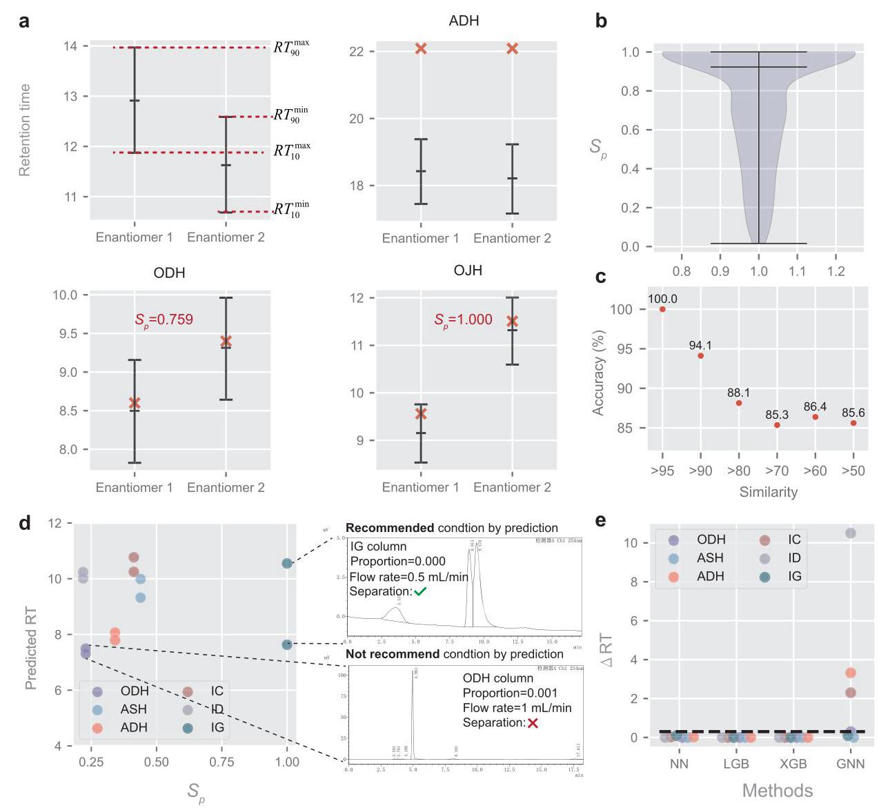
Fig. 6 | Definition and application of Chromatographic enantioseparation probability assessment. a The definition of separation probability and some examples under different conditions, including an inseparable situation under the ADH column and two separate situations under ODH and OJH columns. The red cross refers to the observed data while the lines in error bar refers to 90th quantile, predicted retention time (RT), and 10th quantile, respectively, which are predicted by the model. b The violin plot of the distribution of calculated ${S}_{p}$ for 412 pairs of testing enantiomers. The black lines mean the maximum, median, and minimum values, respectively. c The accuracy of enantioseparation prediction for the enan-tiomers with different thresholds of similarities. d An example of the utilization in practical application, including prediction of retention time and ${S}_{p}$ for the same enantiomers under different columns made by multi-column prediction model (left), and verification experiments (right). ${S}_{p}$ refers to the separation probability. e The $\bigtriangleup {RT}$ for each of the candidate conditions with four conventional ML methods. The dark dotted line refers to the separation threshold. Source data are provided as a Source Data file.

图6 | 色谱对映体分离概率评估的定义与应用。a分离概率的定义以及不同条件下的一些示例，包括在ADH柱下的不可分离情况以及在ODH和OJH柱下的两种分离情况。红色十字表示观测数据，误差条中的线分别表示由模型预测的第90百分位数、预测保留时间(RT)和第10百分位数。b 412对测试对映体的计算${S}_{p}$分布的小提琴图。黑线分别表示最大值、中位数和最小值。c不同相似度阈值下对映体分离预测的准确性。d实际应用中的一个示例，包括多柱预测模型对同一对映体在不同柱下的保留时间和${S}_{p}$的预测(左)以及验证实验(右)。${S}_{p}$指分离概率。e使用四种传统机器学习方法对每个候选条件的$\bigtriangleup {RT}$。暗虚线表示分离阈值。源数据作为源数据文件提供。

Discussion

讨论

In this work, a research framework is proposed to incorporate machine learning techniques into the field of experimental chemistry to promote the efficiency of the researchers practically when faced with chromatographic enantioseparation. The proposed framework of quantile geometry-enhanced graph neural network (QGeoGNN) focuses on addressing several core issues including data acquisition, chiral molecular 3D representations, and data uncertainty. Firstly, Benefiting from the consistency of standardized commercial HPLC columns, this work manages to construct a chiral molecular retention time dataset from numerous articles in the area of asymmetric catalysis and thus solve the problem of data acquisition. Secondly, a specialized graph neural network called QGeoGNN is established by incorporating molecular 3D conformation, experimental conditions, relevant descriptors, and quantile learning to be more suitable for experimental practice. Considering that the experimental results inherently have uncertainty, the quantile learning technique attempts to capture the uncertainty during the training process and can provide a value range. Thirdly, domain knowledge like chromatographic process equation and HPLC column features is combined with machine learning techniques to further improve the predictive performance of the model. Finally, separation probability is defined in this work to measure the predictive probability of enantiomers being separated under a given condition to facilitate chromatographic enantioseparation.

在本研究中，我们提出了一个研究框架，将机器学习技术引入实验化学领域，以切实提高研究人员在面对色谱对映体分离时的工作效率。所提出的分位数几何增强图神经网络(QGeoGNN)框架专注于解决几个核心问题，包括数据采集、手性分子的3D表示以及数据不确定性。首先，受益于标准化商业HPLC柱的一致性，本研究成功地从不对称催化领域的大量文章中构建了一个手性分子保留时间数据集，从而解决了数据采集问题。其次，通过结合分子3D构象、实验条件、相关描述符和分位数学习，建立了一个名为QGeoGNN的专门图神经网络，使其更适合实验实践。考虑到实验结果本身具有不确定性，分位数学习技术试图在训练过程中捕捉不确定性，并能提供一个值范围。第三，将色谱过程方程和HPLC柱特征等领域知识与机器学习技术相结合，进一步提高模型的预测性能。最后，本研究定义了分离概率，以衡量对映体在给定条件下被分离的预测概率，便于色谱对映体分离。

Experiments have confirmed that the QGeoGNN has a satisfactory ability to predict the retention time of chiral molecules in single-column and multi-column predictions. Furthermore, the QeoGNN can predict the separation probability in diversified conditions quickly and flexibly, and recommend suitable conditions by comparison, which will promote the efficiency of chromatographic enantioseparation.

实验证实，QGeoGNN在单柱和多柱预测中对手性分子保留时间具有令人满意的预测能力。此外，QeoGNN能够快速灵活地预测多种条件下的分离概率，并通过比较推荐合适的条件，这将提高色谱对映体分离的效率。

At present, this research remains some shortcomings that can be improved in the future. Firstly, the representativeness and quality of the data are uncontrolled and sometimes biased since they are extracted from existing literature, which will affect the predictive performance of the machine learning model. Second, due to the lack of repeated test data reported in the literature for the same molecule, data uncertainty is learned from similar molecules. Third, prediction accuracy still needs to be improved when faced with unfamiliar molecules with low similarity. Lastly, the feature extraction process could be further optimized to better represent chiral-related information. Despite these limitations, we believe that this framework has significant potential to facilitate the experimental process by enabling more efficient and effective determination of proper experimental conditions in chromatographic enantioseparation.

目前，本研究仍存在一些不足之处，未来可以改进。首先，由于数据是从现有文献中提取的，其代表性和质量不受控制，有时存在偏差，这将影响机器学习模型的预测性能。其次，由于文献中缺乏同一分子的重复测试数据，数据不确定性是从相似分子中学习的。第三，面对相似性较低的陌生分子时，预测准确性仍需提高。最后，特征提取过程可以进一步优化，以更好地表示手性相关信息。尽管存在这些局限性，但我们相信，该框架通过在色谱对映体分离中更高效、有效地确定合适的实验条件，具有显著的潜力来促进实验过程。

Methods

方法

The graph representation for molecules

分子的图表示

In this work, the molecular representation is accomplished by constructing two graphs, Graph G and H (Fig. 2a). In data science, graphs are often used to describe unstructured data like social networks, chemical molecules, and traffic networks. A typical graph is composed of several nodes and edges that indicate the connection relationship. As illustrated in Fig. 2a, Graph G expresses the plane structure of the chemical molecule where the nodes refer to the atoms and the edges refer to the chemical bonds. The feature of each node in Graph G contains 9 properties of the corresponding atom, including the atomic number, chiral tag, degree, explicit valence, formal charge, hybridization, implicit valence, aromaticity, and the number of connected hydrogen atoms. The feature of each edge in Graph G contains 3 properties of the corresponding bond including bond direction, bond type, and whether in the ring or not. In this work, the experimental condition, elution proportion, is also added to the feature of each bond. On the other hand, Graph H describes the 3D conformation of the molecule where nodes refer to the bond and edges refer to the bond angle (Fig. 2a). The feature of each node in Graph H contains only one property, the length of the corresponding bond, while the feature of each edge in Graph H contains six properties including the bond angle and five relevant descriptors, namely total polar surface area (TPSA), relative polar surface area (RPSA), relative hydrophobic surface area (RASA), molecular distance edge (MEDC), and moran coefficient (MATS). The molecular descriptors are calculated by the python package Mordred and chosen according to the spearman coefficient that identifies the correlation with retention time. In multi-column prediction, the features of HPLC columns are incorporated in the edge feature of Graph G.

在这项工作中，分子表示是通过构建两个图，即图G和图H来完成的(图2a)。在数据科学中，图经常被用来描述非结构化数据，如社交网络、化学分子和交通网络。一个典型的图由几个节点和边组成，这些节点和边表示连接关系。如图2a所示，图G表示化学分子的平面结构，其中节点表示原子，边表示化学键。图G中每个节点的特征包含相应原子的9个属性，包括原子序数、手性标签、度、显价、形式电荷、杂化、隐价、芳香性和连接氢原子的数量。图G中每条边的特征包含相应化学键的3个属性，包括键方向、键类型以及是否在环中。在这项工作中，实验条件洗脱比例也被添加到每条化学键的特征中。另一方面，图H描述了分子的三维构象，其中节点表示化学键，边表示键角(图2a)。图H中每个节点的特征只包含一个属性，即相应化学键的长度，而图H中每条边的特征包含六个属性，包括键角和五个相关描述符，即总极性表面积(TPSA)、相对极性表面积(RPSA)、相对疏水表面积(RASA)、分子距离边(MEDC)和莫兰系数(MATS)。分子描述符由python包Mordred计算，并根据与保留时间的相关性的斯皮尔曼系数进行选择。在多柱预测中，HPLC柱的特征被纳入图G的边特征中。

Details for QGeoGNN

QGeoGNN的详细信息

The optimization of the graph neural network (GNN) is accomplished based on the message-passing mechanism. Specifically, for node $i$ , its representation vector ${h}_{i}^{k}$ at the ${k}^{\text{ th }}$ iteration can be written as:

图神经网络(GNN)的优化是基于消息传递机制完成的。具体来说，对于节点$i$，其在${k}^{\text{ th }}$次迭代时的表示向量${h}_{i}^{k}$可以写成:

Here, ${A}^{k}$ and ${C}^{k}$ are the aggregation function and the update function in the $k$ th iteration. They function as aggregating messages from a node neighborhood and updating the node representation ${}^{16}$ . $N\left( i\right)$ is the neighborhood of node $i$ , and ${x}_{ij}$ is the edge that connects node $i$ and its neighborhood node $j$ . In the final iteration, the readout function, i.e., the pooling function, is employed to obtain the graph representation ${h}_{G}$ from the node representations in the final iteration $K$ . The formula can be expressed as:

这里，${A}^{k}$和${C}^{k}$是第$k$次迭代中的聚合函数和更新函数。它们的作用是聚合来自节点邻域的消息并更新节点表示${}^{16}$。$N\left( i\right)$是节点$i$的邻域，${x}_{ij}$是连接节点$i$及其邻域节点$j$的边。在最后一次迭代中，使用读出函数，即池化函数，从最后一次迭代$K$中的节点表示中获得图表示${h}_{G}$。公式可以表示为:

where $R$ is the readout function and $/$ is the collection of all nodes in the graph. In this work, the readout function is the summation.

其中$R$是读出函数，$/$是图中所有节点的集合。在这项工作中，读出函数是求和。

The GeoGNN proposed in this work involves the massage passing in two graphs, Graph H and G, simultaneously. Therefore, its optimization mechanism is a little more complex, which is detailed in this section. In GeoGNN, the node representations in Graph H are first calculated in the same way as Eq. (6), which can be formalized as:

这项工作中提出的GeoGNN同时涉及在两个图Graph H和G中进行消息传递。因此，其优化机制稍微复杂一些，将在本节详细介绍。在GeoGNN中，首先以与式(6)相同的方式计算图H中的节点表示，其形式化表示为:

where ${H}_{i}$ and ${H}_{j}$ are the node $i, j$ in Graph H. Considering that the node of Graph H and the edge of Graph G are both related to the bonds of the molecules, a bridge that transforms information between Graph H and G is constructed. Therefore, the node representations in the Graph G are obtained in consideration of the ${h}_{{H}_{i}}^{k - 1}$ , which is written as:

其中${H}_{i}$和${H}_{j}$是图H中的节点$i, j$。考虑到图H的节点和图G的边都与分子的键有关，构建了一个在图H和G之间转换信息的桥梁。因此，考虑${h}_{{H}_{i}}^{k - 1}$来获得图G中的节点表示，其写成:

It can be seen that the information of Graph H is incorporated into the node representations of Graph G. Then, the readout function is conducted to obtain the graph representation of QGeoGNN as:

可以看出，图H的信息被纳入到图G的节点表示中。然后，进行读出函数以获得QGeoGNN的图表示为:

In this way, the information of 3D conformation for the molecule including the bond length and bond angle is incorporated into the QGeoGNN to get a graph representation that can distinguish the enantiomers. Considering that the ${h}_{\text{ Graph }}$ is a vector with the dimension of embedding size, a fully connected layer is adopted to transform the graph representation into the prediction.

通过这种方式，包括键长和键角在内的分子三维构象信息被纳入到QGeoGNN中，以获得能够区分对映体的图表示。考虑到${h}_{\text{ Graph }}$是一个具有嵌入大小维度的向量，采用全连接层将图表示转换为预测结果。

Quantile geometry-enhanced graph neural network (QGeoGNN)

分位数几何增强图神经网络(QGeoGNN)

The QeoGNN is constructed based on the graph representation and the graph isomorphism network (GIN). The fundament of GIN is the graph isomorphic convolution layer (GINConv) ${}^{37}$ , which is defined as:

QeoGNN基于图表示和图同构网络(GIN)构建。GIN的基础是图同构卷积层(GINConv)${}^{37}$，其定义为:

where ${x}_{i}^{\prime }$ and ${x}_{i}$ are the node representations in the next layer and current layer, respectively. ${x}_{j}$ is the representation in the adjacent nodes. ${h}_{\theta }$ is a multilayer perceptron (MLP) and $\varepsilon$ is a constant that equals 0 in this work. In the QGeoGNN, the node embedding is performed for each node in Graph H to obtain the corresponding node representation based on GINConv. Then, the node representation of Graph $\mathrm{H}$ is added to the edge representation of Graph $\mathrm{G}$ to build a bridge for information transmission between Graph G and Graph H. Afterwards, the node representation of each node in Graph G obtained by node embedding is pooled to get the graph representation. Finally, a fully-connected layer is used to transform the graph representation into the prediction. Deep quantile learning is incorporated into the QGeoGNN by modifying the loss function.

其中${x}_{i}^{\prime }$和${x}_{i}$分别是下一层和当前层的节点表示。${x}_{j}$是相邻节点中的表示。${h}_{\theta }$是多层感知器(MLP)，$\varepsilon$是在本工作中等于0的常数。在QGeoGNN中，基于GINConv对图H中的每个节点进行节点嵌入以获得相应的节点表示。然后，将图$\mathrm{H}$的节点表示添加到图$\mathrm{G}$的边表示中，以构建图G和图H之间信息传输的桥梁。之后，对通过节点嵌入获得的图G中每个节点的节点表示进行池化以获得图表示。最后，使用全连接层将图表示转换为预测。通过修改损失函数将深度分位数学习纳入QGeoGNN。

Benefiting from the deep quantile learning technique employed in this work, the quantiles of the prediction that is seen as a variable can be obtained. In this work, we choose the 90th quantile and 10th quantile as the upper and lower bound to measure the uncertainty of the predicted RTv. Therefore, the output neuron of the fully-connected layer is 3 . The quantile learning is accomplished by the quantile loss in the loss function, which is written as

受益于本工作中采用的深度分位数学习技术，可以获得被视为变量的预测分位数。在本工作中，我们选择第90分位数和第10分位数作为上下界来衡量预测RTv的不确定性。因此，全连接层的输出神经元为3。分位数学习通过损失函数中的分位数损失来完成，其写为

$$

• \frac{1}{N}\mathop{\sum }\limits_{{i = 1}}^{N}\operatorname{ReLu}\left( {{y}{i}^{10} - {y}{i}^{\text{ pred }}}\right) + \frac{1}{N}\mathop{\sum }\limits_{{i = 1}}^{N}\operatorname{ReLu}\left( {{y}{i}^{\text{ pred }} - {y}{i}^{90}}\right) \tag{15} $$

$$

• \frac{1}{N}\mathop{\sum }\limits_{{i = 1}}^{N}\operatorname{ReLu}\left( {2 - {y}_{i}^{\text{ pred }}}\right) \text{ . } $$

The loss function is composed of three parts including the quantile loss, quantile limit, and deadtime limit. The quantile loss function is defined in Eq. (2). The essence of quantile loss is a segmented function, which separates overestimated and underestimated cases and gives different coefficients. Through the quantile loss, the different quantiles of the target value can be learned during training. It is worth noting that the mean squared error is utilized in predicting the RT $v$ instead of the mean absolute error in conventional quantile learning because we find that it is more suitable for the optimization of the geometry-enhanced graph neural network. Meanwhile, some physical and mathematical constraints, including quantile relationships and the dead time limit. For example, the relationship ${y}^{10} \leq {y}^{\text{ pred }} \leq {y}^{90}$ should be satisfied. In the HPLC column, dead time refers to the retention time of components that do not interact with fixation, which is the lower bound of the retention time (RT). In this work, the deadtime limit of RT $v$ is 2, which is decided based on the analysis of the datasets. These constraints in the loss function can avoid the QGeoGNN to make predictions that do not conform to physical and mathematical laws, which improves its accuracy and confidence.

损失函数由分位数损失、分位数限制和死时间限制三部分组成。分位数损失函数在式(2)中定义。分位数损失的本质是一个分段函数，它区分高估和低估情况并给出不同的系数。通过分位数损失，可以在训练期间学习目标值的不同分位数。值得注意的是，在预测RT$v$时使用均方误差而不是传统分位数学习中的平均绝对误差，因为我们发现它更适合几何增强图神经网络的优化。同时，一些物理和数学约束，包括分位数关系和死时间限制。例如，应满足关系${y}^{10} \leq {y}^{\text{ pred }} \leq {y}^{90}$。在HPLC柱中，死时间是指不与固定相相互作用的组分的保留时间，它是保留时间(RT)的下限。在本工作中，RT$v$的死时间限制为2，这是根据数据集分析确定的。损失函数中的这些约束可以避免QGeoGNN做出不符合物理和数学规律的预测，从而提高其准确性和可信度。

The incorporation of column information

柱信息的纳入

For multi-column prediction, the column information is incorporated into the QGeoGNN. In this section, the details for the incorporation of column information are detailed. As illustrated in Fig. 4b, QGeoGNN involves two graphs, the atom-bond graph (Graph G) and the bond-angle graph (Graph H). In the graph neural network, the graph structure is described in the form of the adjacent matrix (Fig. 2a). Considering that the adjacent matrix is usually sparse, a compact form called the coordinate matrix (COO matrix) is adapted to represent the sparse matrix to improve storage and computing efficiency. Therefore, the edge index of a graph can be represented in the form of a COO matrix with the size of [2, num_messages]. The variable num_messages refers to the number of massage paths, which normally equals the number of edges. The feature of each edge corresponds to a relevant vector that incorporates several important attributes. Therefore, the feature for all edges can be expressed by a matrix with the size of [num_messages, num_features], where the variable of num_features refers to the number of relevant attributes. In the multi-column prediction, the connection type, substrates, and packing material size are incorporated into the edge features in Graph G. The properties of CSPs are described by relevant descriptors and are added to the edge features in Graph H. As illustrated in Fig. 4b, the edge feature of Graph G turns to be the size of [num_messages_G, 7] by adding the attributes of the column’s properties, including the packing material size, substrates (cellulose or amylose), and connection type (immobilized or coated), and each of them is represented by a vector with the size of [num_messages_G, 1]. Of note, the substrate is digitized by 0 (amylose) and 1 (cellulose), and the connection type is digitized similarly by 0 (immobilized) and 1 (coated). Similarly, the column descriptors (CSP descriptors) are incorporated into Graph H to augment the feature matrix to the size of [num_messages_H, 11]. In this work, the graph neural network (GNN) with merely graph G is employed for comparison. Therefore, for GNN, all column information including the column’s outer features and descriptors are added to the edge feature matrix of Graph G along with the molecular descriptors to generate a matrix with the size of [num_messages_H, 17].

对于多柱预测，柱信息被纳入QGeoGNN。在本节中，详细介绍了纳入柱信息的细节。如图4b所示，QGeoGNN涉及两个图，原子-键图(图G)和键角图(图H)。在图神经网络中，图结构以邻接矩阵的形式描述(图2a)。考虑到邻接矩阵通常是稀疏的，采用一种称为坐标矩阵(COO矩阵)的紧凑形式来表示稀疏矩阵，以提高存储和计算效率。因此，图的边索引可以用大小为[2, num_messages]的COO矩阵形式表示。变量num_messages指的是消息路径的数量，通常等于边的数量。每条边的特征对应一个包含几个重要属性的相关向量。因此，所有边的特征可以用大小为[num_messages, num_features]的矩阵表示，其中变量num_features指的是相关属性的数量。在多柱预测中，连接类型、底物和填充材料尺寸被纳入图G的边特征中。CSP的属性由相关描述符描述，并添加到图H的边特征中。如图4b所示，通过添加柱属性的属性，包括填充材料尺寸、底物(纤维素或直链淀粉)和连接类型(固定化或涂层)，图G的边特征变为大小为[num_messages_G, 7]，并且它们中的每一个都由大小为[num_messages_G, 1]的向量表示。值得注意的是，底物用0(直链淀粉)和1(纤维素)数字化，连接类型类似地用0(固定化)和1(涂层)数字化。同样，柱描述符(CSP描述符)被纳入图H，以将特征矩阵扩充到大小为[num_messages_H, 11]。在这项工作中，仅使用图G的图神经网络(GNN)进行比较。因此，对于GNN，所有柱信息，包括柱的外部特征和描述符，都与分子描述符一起添加到图G的边特征矩阵中，以生成大小为[num_messages_H, 17]的矩阵。

Automatic construction of the CMRT dataset

CMRT数据集的自动构建

In this work, a chiral molecular retention time (CMRT) dataset is established by extracting experimental outcomes from 644 articles about asymmetric catalysis. The dataset constitutes the retention time of 25,847 molecules, which contains 11,720 pairs of enantiomers, experimental information, and HPLC column information. The basic flows of constructing the dataset involve several major steps, including determining the data sources, downloading the supplementary information, converting the format, extracting the information, and preprocessing the data. First, 18 research groups that are committed to the research of asymmetric catalysis for years are considered to be the data sources. Then, the supplementary information of relevant articles (644 articles) is downloaded from the journal websites successively and manually. Afterward, the pages of HPLC experimental reports in each article are extracted and converted to text format (.txt). The converted texts from each article are copied and combined into a separate text file. Benefitting from the similar format of reporting the experimental outcomes in the literature of asymmetric catalysis, the experimental results can be extracted automatically through natural language processing techniques, which is detailed below. Finally, the extracted data are pre-processed to obtain the formatted data, where rapid verification is conducted manually to exclude data with obvious errors caused in the extraction process.

在本工作中，通过从644篇关于不对称催化的文章中提取实验结果，建立了一个手性分子保留时间(CMRT)数据集。该数据集包含25,847个分子的保留时间，其中包括11,720对对映体、实验信息和高效液相色谱(HPLC)柱信息。构建数据集的基本流程涉及几个主要步骤，包括确定数据源、下载补充信息、转换格式、提取信息和预处理数据。首先，将多年来致力于不对称催化研究的18个研究小组视为数据源。然后，从期刊网站上依次手动下载相关文章(644篇)的补充信息。之后，提取每篇文章中HPLC实验报告的页面并转换为文本格式(.txt)。将每篇文章转换后的文本复制并合并到一个单独的文本文件中。得益于不对称催化文献中报告实验结果的格式相似，可以通过自然语言处理技术自动提取实验结果，具体如下所述。最后，对提取的数据进行预处理以获得格式化数据，在此过程中进行人工快速验证以排除提取过程中产生的明显错误数据。

Benefitting from the similar format of reporting the experimental outcomes in the literature of asymmetric catalysis, we can extract the data automatically. A typical experimental report in the article is provided in Supplementary Figure. 1 as an example ${}^{38}$ . This experimental report is usually placed in the supplementary materials of the relevant literature, which have been downloaded beforehand. For each reported chiral molecule, there will exist a corresponding experimental report. A program is written to extract data automatically and the principle is detailed below. As shown in Supplementary Fig. 1a, the molecular name is located by the word (S) or (R), which indicates that the compound is a chiral molecule with fixed conformation. After extracting the molecular name, the verification word ‘HPLC’ is utilized to decide whether this report employs the HPLC to recognize the molecule. If not, the report will be dropped and the subsequent one will be considered. When satisfying the demand of the verification word, all relevant information is extracted step by step including column type, elution proportion, flow rate, the retention time for this conformer, and its enantiomer by corresponding keywords (Supplementary Fig. 1b).

得益于不对称催化文献中报告实验结果的格式相似，我们可以自动提取数据。补充图1中提供了文章中的一份典型实验报告作为示例${}^{38}$。这份实验报告通常放在相关文献的补充材料中，这些材料已事先下载。对于每个报告的手性分子，都会有相应的实验报告。编写了一个程序来自动提取数据，原理如下所述。如补充图1a所示，通过单词(S)或(R)定位分子名称，这表明该化合物是具有固定构象的手性分子。提取分子名称后，利用验证词“HPLC”来确定该报告是否采用HPLC来识别分子。如果不是，则放弃该报告并考虑下一个。当满足验证词的要求时，通过相应的关键词逐步提取所有相关信息，包括柱类型、洗脱比例、流速、该构象异构体及其对映体的保留时间(补充图1b)。

The extracted raw data are saved in csv format. After the raw data are obtained, further treatment is conducted to extract the simplified column name from the column type, and convert the proportion to the ratio. For example, the elution proportion in Supplementary Fig. 1 (98/ 02) will be transformed into 0.02. Considering that the report only includes two retention times (major and minor), we only contain the molecules with less than two chiral centers since the retention times and enantiomers can be matched easily. The extracted names of enantiomers are converted into SMILES through a website (https:// cactus.nci.nih.gov/chemical/structure). Specifically, an automatic program written by Python is employed to open the URL that converts molecule names to SMILES. For example, to obtain the SMILEs of D-Lactose, the program will open the URL https://cactus.nci.nih.gov/ chemical/structure/D-Lactose/smiles and read the converted SMILES. Other molecule names can be obtained in the same manner by replacing the ‘D-Lactose’ with the molecule’s name in the above URL.

提取的原始数据以csv格式保存。获得原始数据后，进行进一步处理，从柱类型中提取简化的柱名称，并将比例转换为比率。例如，补充图1中的洗脱比例(98/02)将转换为0.02。考虑到报告仅包括两个保留时间(主要和次要)，我们只包含手性中心少于两个的分子，因为保留时间和对映体可以很容易地匹配。通过一个网站(https://cactus.nci.nih.gov/chemical/structure)将提取的对映体名称转换为SMILES。具体来说，使用Python编写的自动程序打开将分子名称转换为SMILES的URL。例如，为了获得D-乳糖的SMILES，程序将打开URL https://cactus.nci.nih.gov/chemical/structure/D-Lactose/smiles并读取转换后的SMILES。通过在上述URL中用分子名称替换“D-乳糖”，可以以相同的方式获得其他分子名称的SMILES。

Experimental verification of chromatographic process equation

色谱过程方程的实验验证

In this work, in order to reduce the variable considered in retention time prediction, the chromatographic process equation is considered to construct the relationship between the retention time and the speed, which is written in Eq. (1). Therefore, under a fixed experimental condition where the $K,{V}_{m}$ , and ${V}_{s}$ are fixed, the retention time for the molecule and the flow rate is inversely proportional related. Therefore, in this work, the prediction target is set to be RT $\times v$ , which is abbreviated as RT $v$ . In this section, the chromatographic process equation is verified by an experiment which is illustrated in Supplementary Fig. 4. In the verification, the retention times (RT) of a pair of enantiomers with different flow rates $v$ are measured in the laboratory. The experimental condition is the IG column with elution proportion=0.001. In some situations, the outcome is measured repeatedly. The fitted curve and observed retention times are illustrated in Supplementary Fig. 4a. It is discovered that the chromatographic process equation functions well when the flow rate is not so small (bigger than 0.2). Fortunately, there are only smaller than 0.5% data where the flow rate is smaller than 0.2, which means that most data in the dataset satisfies the chromatographic process equation. Therefore, it is rational to incorporate the chromatographic process equation into QGeoGNN to satisfy the underlying relationship between the retention time and the speed and facilitate model construction.

在本工作中，为了减少保留时间预测中考虑的变量，考虑使用色谱过程方程来构建保留时间与速度之间的关系，如式(1)所示。因此，在固定的实验条件下，当$K,{V}_{m}$和${V}_{s}$固定时，分子的保留时间与流速成反比关系。因此，在本工作中，预测目标设定为RT $\times v$，简称为RT $v$。在本节中，通过实验验证了色谱过程方程，实验情况见补充图4。在验证过程中，在实验室中测量了一对对映体在不同流速$v$下的保留时间(RT)。实验条件是洗脱比例 = 0.001的IG柱。在某些情况下，会重复测量结果。拟合曲线和观察到的保留时间见补充图4a。发现当流速不是太小(大于0.2)时，色谱过程方程运行良好。幸运的是，数据集中流速小于0.2的数据仅占不到0.5%，这意味着数据集中的大多数数据都满足色谱过程方程。因此，将色谱过程方程纳入QGeoGNN以满足保留时间与速度之间的潜在关系并促进模型构建是合理的。

According to the chromatographic process equation and the above experiments in the laboratory, the RTv should keep constant with different flow rates when other experimental conditions are fixed. Nevertheless, considering that data in the CMRT dataset are collected from various literature, errors will emerge in the RTv model because of the difference between the experimental environment of diversified laboratories. Therefore, the scalability of the proposed RT $v$ model in the dataset is further investigated. Here, 364 pairs of the same enantiomer acquired in different flow rates are selected from the CMRT dataset, where the flow rates range from ${0.3}\mathrm{\;{mL}}/\mathrm{{min}}$ to $1\mathrm{\;{mL}}/\mathrm{{min}}$ and the retention time range from ${3.5}\mathrm{\;{min}}$ to ${60}\mathrm{\;{min}}$ . Most of these enantiomers are measured in multiple laboratories independently. In order to measure the error range of the RT $v$ model, the absolute error of the calculated RT $v$ for the same pair of enan-tiomers in different flow rates is obtained and analyzed. The violin plot of the error distribution is displayed in Supplementary Fig. 4b. The median error is 1.37. It is discovered that there exists a certain degree of error in the RT $v$ model but most of them are small. Meanwhile, the existence of a few samples with extremely large errors implies that there may be a few exceptions to the chromatographic process equation or mistakes in the data.

根据色谱过程方程和上述实验室实验，当其他实验条件固定时，RTv应随不同流速保持恒定。然而，考虑到CMRT数据集中的数据是从各种文献中收集的，由于不同实验室的实验环境差异，RTv模型中会出现误差。因此，进一步研究了所提出的RT $v$模型在数据集中的可扩展性。这里，从CMRT数据集中选择了364对在不同流速下获得的相同对映体，其中流速范围从${0.3}\mathrm{\;{mL}}/\mathrm{{min}}$到$1\mathrm{\;{mL}}/\mathrm{{min}}$，保留时间范围从${3.5}\mathrm{\;{min}}$到${60}\mathrm{\;{min}}$。这些对映体中的大多数是在多个实验室独立测量的。为了测量RT $v$模型的误差范围，获取并分析了同一对对映体在不同流速下计算得到的RT $v$的绝对误差。误差分布的小提琴图见补充图4b。中位数误差为1.37。发现RT $v$模型中存在一定程度的误差，但大多数误差较小。同时，存在一些误差极大的样本，这意味着色谱过程方程可能存在一些例外情况或数据存在错误。

Derivation of chromatographic separation probability

色谱分离概率的推导

In this work, a measurement denoted as chromatographic separation probability ${S}_{p}$ is defined to measure the probability that the ML model would correctly separate the enantiomers under the specific experimental setting. In this section, the definition and derivation of chromatographic separation probability are detailed. Benefiting from the proposed QGeoGNN, the value range of the enantiomers’ retention time can be obtained. The definition of chromatographic separation probability ${S}_{p}$ is defined based on the naïve principle that the area within the overlapping part of the value range is considered inseparable, while other areas are separable. Therefore, the definition of ${S}_{p}$ can be written as Eq. (4). In order to derive the formula of ${S}_{p}$ , two typical scenarios are discussed. The example is illustrated in Supplementary Fig. 7. For the situation in Supplementary Fig. 7a where the value ranges of enantiomers are partially overlapped, the overlapping region is predicted to be inseparable while other regions are seen as separable. Therefore, in this situation, ${L}_{\text{ separable }}$ and ${L}_{\text{ total }}$ can be calculated as

在本研究中，定义了一种名为色谱分离概率${S}_{p}$的度量，用于衡量机器学习模型在特定实验设置下正确分离对映体的概率。在本节中，将详细介绍色谱分离概率的定义和推导过程。受益于所提出的QGeoGNN，可以获得对映体保留时间的取值范围。色谱分离概率${S}_{p}$的定义基于一个简单的原则:取值范围重叠部分内的区域被视为不可分离，而其他区域是可分离的。因此，${S}_{p}$的定义可以写成公式(4)。为了推导${S}_{p}$的公式，讨论了两种典型情况。示例见补充图7。对于补充图7a中对映体取值范围部分重叠的情况，重叠区域被预测为不可分离，而其他区域被视为可分离。因此，在这种情况下，${L}_{\text{ separable }}$和${L}_{\text{ total }}$可以计算为

the ${S}_{p}$ can be derived as

${S}_{p}$可以推导为

Here, $R{T}_{90}^{\max }$ and $R{T}_{90}^{\min }$ are the maximum and minimum of 90th percentiles for both enantiomers, $R{T}_{10}^{\max }$ and $R{T}_{10}^{\min }$ are the maximum and minimum of 10th percentiles, respectively. For a special case where the value ranges of enantiomers are completely overlapped, ${S}_{p}$ will be equal to 0 since the ${L}_{\text{ separable }} = 0$ . For the situation in Supplementary Fig. 7b where the value ranges of enantiomers are disjoint. It is obvious that the enantiomers are predicted to be separable within the range of error, and the ${S}_{\mathrm{p}} = 1$ . In general, the ${S}_{p}$ can be summarized as

这里，$R{T}_{90}^{\max }$和$R{T}_{90}^{\min }$分别是两种对映体第90百分位数的最大值和最小值，$R{T}_{10}^{\max }$和$R{T}_{10}^{\min }$分别是第10百分位数的最大值和最小值。对于对映体取值范围完全重叠的特殊情况，由于${L}_{\text{ separable }} = 0$，${S}_{p}$将等于0。对于补充图7b中对映体取值范围不相交的情况。很明显，在误差范围内预测对映体是可分离的，并且${S}_{\mathrm{p}} = 1$。一般来说，${S}_{p}$可以总结为

which can be simplified as

可以简化为

Therefore, the defined chromatographic separation probability ${S}_{p}$ ranges from 0 to 1 . A higher ${S}_{p}$ refers to a larger region of separable, that is, a higher possibility that the enantiomers are predicted to be separable by the QGeoGNN.

因此，定义的色谱分离概率${S}_{p}$的范围是0到1。${S}_{p}$越高，表示可分离区域越大，即通过QGeoGNN预测对映体可分离的可能性越高。

Experimental settings and parameters

实验设置和参数

In the QGeoGNN utilized in this work, the number of GINConv is 5 , the graph pooling strategy is the summation, the embedding dimension of the node and edge representation is 128 , and the batch size is 2048 . The training epoch is 1500 , and the validate loss is adapted for early stopping. The optimizer is Adam and the learning rate is 0.001 . For single-column prediction, the prediction models are established for ADH, ODH, IC, and IA columns, respectively. For each column, the sub-dataset is randomly divided into ${90}/5/5$ to obtain the training, validating, and testing dataset. For multi-column prediction, the entire dataset is split into 90/5/5 to train a synthetic model. For comparison, the XGB, LGB, ANN, and GNN are also employed to train a predictive model. The input of XGB, LGB, and ANN is composed of the 167- dimensional MACCS keys that are utilized to represent the molecular structure, the 5-dimensional molecular descriptors that are the same as those utilized in QGeoGNN, and 3-dimensional column information. For XGB, the number of estimators is 200, the maximum depth is 3, and the learning rate is chosen to be 0.1 . For LGB, the maximum depth is 5 , the learning rate is 0.007 , the number of leaves is 25 , and the number of estimators is 1000. For ANN, there are 3 hidden layers with 50 hidden neurons in each hidden layer. The activation function is leaky ReLu and the optimizer is Adam with a learning rate of 0.001 . The training epoch is 10,000 and early stopping is adopted. The construction of GNN is similar to QGeoGNN while it only has Graph G, and the loss function is of the mean squared error between the predicted and observed value. The column information is incorporated into the edge features for GNN.

在本工作中使用的QGeoGNN中，GINConv的数量为5，图池化策略为求和，节点和边表示的嵌入维度为128，批量大小为2048。训练轮数为1500，并采用验证损失进行早期停止。优化器为Adam，学习率为0.001。对于单柱预测，分别为ADH、ODH、IC和IA柱建立预测模型。对于每一列，子数据集被随机划分为${90}/5/5$以获得训练、验证和测试数据集。对于多柱预测，整个数据集按90/5/5拆分以训练一个综合模型。为了进行比较，还采用XGB、LGB、ANN和GNN来训练预测模型。XGB、LGB和ANN的输入由用于表示分子结构的167维MACCS键、与QGeoGNN中使用的相同的5维分子描述符以及3维柱信息组成。对于XGB，估计器的数量为200，最大深度为3，学习率选择为0.1。对于LGB，最大深度为5，学习率为0.007，叶子数为25，估计器的数量为1000。对于ANN，有3个隐藏层，每个隐藏层有50个隐藏神经元。激活函数为leaky ReLu，优化器为Adam，学习率为0.001。训练轮数为10000并采用早期停止。GNN的构建与QGeoGNN类似，但其仅具有图G，损失函数为预测值与观测值之间的均方误差。柱信息被纳入GNN的边特征中。

Reporting summary

报告总结

Further information on research design is available in the Nature Portfolio Reporting Summary linked to this article.

有关研究设计的更多信息，请参阅与此文章相关的《自然》系列报告总结。

Data availability

数据可用性

The CMRT dataset generated in this study have been deposited in the Github repository, https://github.com/woshixuhao/Retention-Time-Prediction-for-Chromatographic-Enantioseparation/tree/main/ dataset. Source data are provided with this paper.

本研究中生成的CMRT数据集已存于Github仓库，https://github.com/woshixuhao/Retention-Time-Prediction-for-Chromatographic-Enantioseparation/tree/main/ dataset。本文提供了源数据。

Code availability

代码可用性

All original code has been deposited at the website https://github.com/ woshixuhao/Retention-Time-Prediction-for-Chromatographic-Enantioseparation/tree/main/code. The version of the record of the GitHub repo is doi:10.5281/zenodo.7623903.

所有原始代码已存放在网站https://github.com/ woshixuhao/Retention-Time-Prediction-for-Chromatographic-Enantioseparation/tree/main/code。GitHub仓库记录的版本为doi:10.5281/zenodo.7623903。

References

参考文献

1. Artrith, N. et al. Best practices in machine learning for chemistry. Nat. Chem. 13, 505-508 (2021).

2. Muratov, E. N. et al. QSAR without borders. Chem. Soc. Rev. 49, 3525-3564 (2020).

3. Gupta, R. et al. Artificial intelligence to deep learning: machine intelligence approach for drug discovery. Mol. Divers. 25 (2021).

4. Ishida, S., Terayama, K., Kojima, R., Takasu, K. & Okuno, Y. Prediction and interpretable visualization of retrosynthetic reactions using graph convolutional networks. J. Chem. Inf. Model. 59, 5026-5033 (2019).

5. Coley, C. W., Green, W. H. & Jensen, K. F. Machine learning in computer-aided synthesis planning. Acc. Chem. Res. 51, 1281-1289 (2018).

6. Shen, Y. et al. Automation and computer-assisted planning for chemical synthesis. Nat. Rev. Methods Prim. 1 (2021).

7. Tkatchenko, A. Machine learning for chemical discovery. Nat. Commun. 11 (2020).

8. Dobbelaere, M. R., Plehiers, P. P., Van de Vijver, R., Stevens, C. V. & Van Geem, K. M. Machine learning in chemical. Eng.: Strengths Weaknesses Opportunities Threats Eng. 7, 5166-5179 (2021).

9. Haghighatlari, M. et al. Learning to make chemical predictions: the interplay of feature representation, data, and machine learning methods. Chem. 6, 1527-1542 (2020).

10. Burger, B. et al. A mobile robotic chemist. Nature 583, 237-241 (2020).

11. Xu, H. et al. High-throughput discovery of chemical structure-polarity relationships combining automation and machine-learning techniques. Chem 8, 1-13 (2022).

12. Xu, H., Zhang, D. & Mo, F. High-throughput automated platform for thin layer chromatography analysis. STAR Protoc. 3, 101893 (2022).

13. Weininger, D. SMILES, a chemical language and information system: 1: introduction to methodology and encoding rules. J. Chem. Inf. Comput. Sci. 28, 31-36 (1988).

14. Rogers, D. & Hahn, M. Extended-connectivity fingerprints. J. Chem. Inf. Model 50, 742-754 (2010).

15. Moriwaki, H., Tian, Y. S., Kawashita, N. & Takagi, T. Mordred: a molecular descriptor calculator. J. Cheminform. 10, 4 (2018).

16. Fang, X. et al. Geometry-enhanced molecular representation learning for property prediction. Nat. Mach. Intell. 4, 127-134 (2022).

17. Zhou, G. et al. Uni-Mol: a universal 3D molecular representation learning framework. ChemRxiv 1-20 (2022).

18. Blaser, H. U. Chirality and its implications for the pharmaceutical industry. Rend. Lincei 24, 213-216 (2013).

19. Brandt, J. R., Salerno, F. & Fuchter, M. J. The added value of small-molecule chirality in technological applications. Nat. Rev. Chem. 1, 6137 (2017).

20. Peluso, P. & Chankvetadze, B. Recognition in the domain of molecular chirality: from noncovalent interactions to separation of enantiomers. Chem. Rev. 122, 13235-13400 (2022).

21. Okamoto, Y. & Ikai, T. Chiral HPLC for efficient resolution of enan-tiomers. Chem. Soc. Rev. 37, 2593-2608 (2008).

22. Sun, L. et al. A simple method for HPLC retention time prediction: linear calibration using two reference substances. Chinese Med. (United Kingdom) 12 (2017).

23. Usman, A. G., Işik, S. & Abba, S. I. A novel multi-model data-driven ensemble technique for the prediction of retention factor in HPLC method development. Chromatographia 83, 933-945 (2020).

24. Osipenko, S. et al. Machine learning to predict retention time of small molecules in nano-HPLC. Anal. Bioanal. Chem. 412, 7767-7776 (2020).

25. Domingo-Almenara, X. et al. The METLIN small molecule dataset for machine learning-based retention time prediction. Nat. Commun. 10, 1-9 (2019).

26. Low, D. Y. et al. Data sharing in PredRet for accurate prediction of retention time: application to plant food bioactive compounds. Food Chem. 357, 129757 (2021).

27. Eriksson, T., Björkman, S. & Höglund, P. Clinical pharmacology of thalidomide. Eur. J. Clin. Pharmacol. 57, 365-376 (2001).

28. Francotte, E. R. Enantioselective chromatography as a powerful alternative for the preparation of drug enantiomers. J. Chromatogr. A 906, 379-397 (2001).

29. Jiang, D. et al. Could graph neural networks learn better molecular representation for drug discovery? A comparison study of descriptor-based and graph-based models. J. Cheminform. 13, 1-23 (2021).

30. Nicoud, R. M. Chromatographic processes: Modeling, simulation and design. Chromatographic Processes: Modeling, Simulation and Design https://doi.org/10.1017/CBO9781139998284 (2015).

31. Hasanzadeh, A. et al. Bayesian graph neural networks with adaptive connection sampling. In Proc. 37th International Conference on Machine Learning, ICML'20. Article No. 383. https://dl.acm.org/ doi/10.5555/3524938.3525321 (JMLR.org, 2020).

32. Abdar, M. et al. A review of uncertainty quantification in deep learning: techniques, applications and challenges. Inf. Fusion 76, 243-297 (2021).

33. Salinas, D., Flunkert, V., Gasthaus, J. & Januschowski, T. DeepAR: probabilistic forecasting with autoregressive recurrent networks. Int. J. Forecast. 36, 1181-1191 (2020).

34. Zhang, W., Quan, H. & Srinivasan, D. An improved quantile regression neural network for probabilistic load forecasting. IEEE Trans. Smart Grid 10, 4425-4434 (2019).

35. Wolfer, A. M. et al. UPLC-MS retention time prediction: a machine learning approach to metabolite identification in untargeted profiling. Metabolomics 12 (2016).

36. Shen, J. & Okamoto, Y. Efficient separation of enantiomers using stereoregular chiral polymers. Chem. Rev. 116, 1094-1138 (2016).

37. Xu, K., Jegelka, S., Hu, W. & Leskovec, J. How powerful are graph neural networks? 7th Int. Conf. on Learning Representations ICLR 2019 1-17 (2019).

38. Pan, Z. et al. Palladium/TY-phos-catalyzed asymmetric intermolecular $\alpha$ -arylation of aldehydes with aryl bromides. Angew. Chem.-Int. 60, 18542-18546 (2021).

Acknowledgements

致谢

The authors thank Prof. Changkun Li at Shanghai Jiao Tong University for invaluable discussions and helpful suggestions. This work is supported by the Natural Science Foundation of China (Grant Nos. 22071004, 21933001, 22150013, received by F.M.).

作者感谢上海交通大学的李长坤教授进行了宝贵的讨论并提供了有益的建议。本工作得到了中国国家自然科学基金(项目编号:22071004、21933001、22150013，由F.M.获得)的支持。

Author contributions

作者贡献

F.M. constructed the chiral molecular retention time (CMRT) dataset. J.L. and H.X. analyzed the data. H.X. performed chemoinformatic and machine learning studies. H.X. and F.M. wrote the manuscript. F.M. conceived the idea and designed the overall research. F.M. and D.Z. supervised the whole project.

F.M.构建了手性分子保留时间(CMRT)数据集。J.L.和H.X.进行了数据分析。H.X.开展了化学信息学和机器学习研究。H.X.和F.M.撰写了手稿。F.M.提出了想法并设计了整体研究。F.M.和D.Z.监督了整个项目。

Competing interests

利益冲突

F.M., H.X., and D.Z. are inventors on a patent application (CN 2023105190181) submitted by Peking University that cover a chiral separation prediction algorithm based on deep learning. J.L. declares no competing interests.

F.M.、H.X. 和 D.Z. 是北京大学提交的一项专利申请(CN 2023105190181)的发明人，该专利申请涵盖了一种基于深度学习的手性分离预测算法。J.L. 声明无利益冲突。

Additional information

其他信息

Supplementary information The online version contains supplementary material available at https://doi.org/10.1038/s41467-023-38853-3.

补充信息 在线版本包含可在https://doi.org/10.1038/s41467-023-38853-3获取的补充材料。

Correspondence and requests for materials should be addressed to Dongxiao Zhang or Fanyang Mo.

有关通信和材料请求，请寄给张东晓或莫凡洋。

Peer review information Nature Communications thanks Xavier Domingo-Almenara, and the other, anonymous, reviewer(s) for their contribution to the peer review of this work. A peer review file is available.

同行评审信息 《自然通讯》感谢哈维尔·多明戈-阿尔梅纳拉以及其他匿名审稿人对本工作同行评审的贡献。可获取同行评审文件。

Reprints and permissions information is available at

可获取重印和许可信息

http://www.nature.com/reprints

Publisher’s note Springer Nature remains neutral with regard to jurisdictional claims in published maps and institutional affiliations.

出版商说明 施普林格·自然对于已发表地图中的管辖权主张和机构隶属关系保持中立。

Open Access This article is licensed under a Creative Commons Attribution 4.0 International License, which permits use, sharing, adaptation, distribution and reproduction in any medium or format, as long as you give appropriate credit to the original author(s) and the source, provide a link to the Creative Commons license, and indicate if changes were made. The images or other third party material in this article are included in the article’s Creative Commons license, unless indicated otherwise in a credit line to the material. If material is not included in the article’s Creative Commons license and your intended use is not permitted by statutory regulation or exceeds the permitted use, you will need to obtain permission directly from the copyright holder. To view a copy of this license, visit http://creativecommons.org/ licenses/by/4.0/.

开放获取 本文受知识共享署名4.0国际许可协议许可，只要您适当引用原作者和来源，提供知识共享许可协议的链接，并表明是否有修改，就允许在任何媒介或格式中使用、共享、改编、分发和复制。本文中的图片或其他第三方材料包含在文章的知识共享许可协议中，除非在材料的版权声明中另有说明。如果材料不包含在文章的知识共享许可协议中，且您的预期用途不受法律法规允许或超出允许的使用范围，您需要直接从版权所有者处获得许可。要查看此许可协议的副本，请访问http://creativecommons.org/licenses/by/4.0/。

© The Author(s) 2023

© 作者 2023