Intelligent Column Chromatography Prediction Model Based on Automation and Machine Learning
中文 / Bilingual · English version
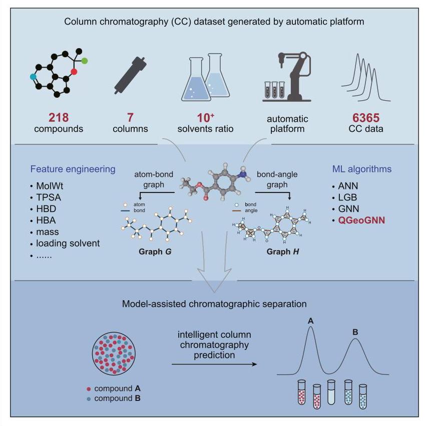
Highlights
Machine learning predicts chromatographic retention via 3D molecular features
Transfer learning enables model adaptation across column specifications
Quantitative separation probability $\left( {S}_{p}\right)$ guides experimental optimization
Data-driven framework reduces empirical trial and error in purification
Authors
Wenchao Wu, Hao Xu, Yang Xu, …, Yan Xu, Dongxiao Zhang, Fanyang Mo
Correspondence
In brief
Chemists traditionally optimize column chromatography through tedious trial and error. This study demonstrates how machine learning models, trained on molecular structures and experimental data, predict compound separation behavior with quantifiable confidence. By translating chemical intuition into computational algorithms, the approach systematically guides purification design-particularly for synthetic intermediates and products. The open-source framework empowers researchers to replace guesswork with data-driven decisions, potentially accelerating chemical discovery while improving reproducibility across laboratories.
Wu et al., 2025, Chem 11, 102598
November 13, 2025 © 2025 Elsevier Inc. All rights are reserved, including those for text and data mining, AI training, and similar technologies. https://doi.org/10.1016/j.chempr.2025.102598
Article
Intelligent column chromatography prediction model based on automation and machine learning
Wenchao Wu, ${}^{1}$ Hao Xu, ${}^{2,3}$ Yang Xu, ${}^{4}$ Peijie Luo, ${}^{4}$ Qingrui Zeng, ${}^{4}$ Yuntian Chen, ${}^{2,3}$ Yan Xu, ${}^{4}$ Dongxiao Zhang, ${}^{2}$ and Fanyang Mo ${}^{1,5,6,7,8, * }$
${}^{1}$ State Key Laboratory of Advanced Waterproof Materials, School of Materials Science and Engineering, Peking University, Beijing 100871, China
${}^{2}$ Zhejiang Key Laboratory of Industrial Intelligence and Digital Twin, Eastern Institute of Technology, Ningbo, Zhejiang 315200, China ${}^{3}$ Ningbo Institute of Digital Twin, Eastern Institute of Technology, Ningbo, Zhejiang 315200, China
${}^{4}$ College of Chemistry and Molecular Engineering, Peking University, Beijing 100871, China
${}^{5}$ School of Advanced Materials, Peking University Shenzhen Graduate School, Shenzhen 518000, China
${}^{6}$ School of AI for Science, Peking University Shenzhen Graduate School, Shenzhen 518000, China
${}^{7}$ Guangdong Provincial Key Laboratory of Nano-Micro Materials Research, Peking University Shenzhen Graduate School, Shenzhen 518000, China
${}^{8}$ Lead contact
*Correspondence:
https://doi.org/10.1016/j.chempr.2025.102598
THE BIGGER PICTURE Column chromatography remains a cornerstone of chemical separation, yet its optimization heavily relies on empirical expertise, leading to inefficiencies and reproducibility challenges across laboratories. This study bridges the gap between traditional practice and data-driven methodologies by establishing a machine learning framework tailored for chromatographic predictions. The integration of automated experimental platforms with the QGeoGNN (quantum geometry-informed graph neural network) algorithm-a model encoding molecular 3D conformations, physicochemical descriptors, and operational parameters-enables systematic retention volume prediction. By employing transfer learning, the framework adapts to diverse column specifications, overcoming the “one-size-fits-all” limitation of conventional approaches. Crucially, the proposed separation probability $\left( {S}_{p}\right)$ quantifies resolution feasibility under target conditions, providing actionable guidance for experimental design.
While the model currently focuses on characterized compounds (e.g., synthetic intermediates and products), its architecture inherently supports expansion to broader chemical spaces as datasets grow. The work highlights two paradigm shifts: (1) transitioning from heuristic trial and error to mechanism-informed optimization and (2) decoupling separation challenges into predictable (known components) versus technology-constrained (unknown impurities) categories. These advances not only accelerate reaction purification workflows but also establish a template for integrating domain knowledge into machine learning pipelines across analytical sciences. Future iterations incorporating temperature effects and stationary phase dynamics could further universalize the framework, while community-driven validation through open-source deployment promises to refine its practical utility. By transforming chromatography from an art to a computational-empirical hybrid discipline, this approach lays groundwork for AI-assisted experimentation in synthetic chemistry and beyond.
SUMMARY
Efficient compound separation remains a persistent challenge in synthetic chemistry, with column chromatography serving as a critical purification tool. Traditional methods require extensive expertise and repetitive labor-areas where AI offers significant advantages. This study introduces an AI-driven platform to automate data collection and optimize separation processes. By leveraging deep learning, the system predicts key separation parameters, while transfer learning enables adaptation to diverse column specifications. A novel metric, separation probability $\left( {S}_{p}\right)$ , quantifies the likelihood of successful component isolation and has been experimentally validated. The approach enhances precision, reduces manual intervention, and expands the scope of chromatographic applications, offering a more efficient and scalable solution for chemical purification.
introduction
Column chromatography (CC) is a crucial tool ${}^{1}$ in modern chemical research, primarily employed for separating and purifying substances. However, traditional CC methods pose significant challenges in terms of efficiency and accuracy, as they often rely on trial-and-error processes and accumulated experience. Even seasoned researchers often spend considerable time experimenting to identify optimal chromatographic conditions, a process typically marked by inefficiency and time consumption. Moreover, the process of CC necessitates a considerable amount of repetitive and physically demanding work, underscoring the urgent need for improvements in this area.
In recent years, the rapid advancement of AI in the field of chemical analysis and process optimization ${}^{2 - 4}$ has opened up new possibilities for improving traditional methods. Due to their powerful expressiveness and ability to accurately model high-dimensional non-linear relationships between variables, data-driven AI methods have shown great potential in the recognition of complex biological samples ${}^{5,6}$ and drug development. ${}^{7,8}$ Chemists have increasingly turned to advanced techniques, including machine learning (ML) and deep learning, to uncover patterns and regularities in complex data, leading to new perspectives and breakthroughs in chemical research. ${}^{9 - {11}}$ In our group, we utilize ML methods in thin-layer chromatography ${\left( \mathrm{{TLC}}\right) }^{{12},{13}}$ and high-performance liquid chromatography ${\left( {HPLC}\right) }^{14}$ to predict the relationship between corresponding chemical structures and their chromatographic retention values. This approach enhances prediction accuracy and reduces experimental workload, providing a more efficient solution for chemical analysis.
From the perspective of a data-driven research paradigm, ML leverages large datasets composed of standardized data. However, despite the fact that CC has been developed for many years, ${}^{1}$ researchers often view it as a tool without systematically collecting experimental conditions and parameters related to the process. Chromatographic datasets often have a large number of missing values and low standardization, which can pose a challenge for further statistic research, even if some data are recorded. Although commercially available automated CC systems save researchers time, they are limited in data collection and device interaction because commercial restrictions prevent open monitoring and automated data processing.
To advance the research and application of CC, it is crucial to develop an intelligent automated platform that not only consistently tests different samples and records standardized data but also includes a recommendation system based on ML algorithms. An automated experimental setup was developed first to collect standardized chromatographic data. Advanced ML algorithms were then used in conjunction with extensive experimental data to train and validate the model. The Al-based chromatography model for predicts and optimizing key parameters in the separation process, such as eluent ratio, solvent type, and column type, are crucial for determining separation efficiency, resolution, and purification quality. By accurately adjusting these parameters, the model can significantly enhance the precision and reliability of chromatographic separations, leading to improved outcomes in both research and industrial applications.
RESULTS
Data acquisition
The research paradigm combining automation with ML technology has already demonstrated its significant advantages in the field of chemical research. This interdisciplinary integration has been successfully applied in various chemical studies, ranging from the optimization of reaction conditions ${}^{15}$ to the interpretation of mechanisms. ${}^{16}$ Through an automated platform, as the research pipeline shown in the Figure 1A, we can systematically collect a large volume of experimental data, and ML technology provides powerful tools to analyze these data, revealing hidden patterns and correlations, thereby deepening our understanding of chemical processes.
In response to the challenges encountered in CC experiments, an automated device was designed in this work for the efficient collection of standard data. The structural design and operational mechanism of the device are depicted in Figure 1B, with a photographic representation provided in Figure S1. The device comprises four independent modules: the pumping unit, which is responsible for eluent infusion and consists of two pumps and a mixer; the injector, which is responsible for sample loading; the UV detector, which is responsible for detecting spectral signal; and the control terminal, which is responsible for handling these modules for synergistic cooperation. A comprehensive description of the operational procedure can be found in the methods section. This hardware support is the foundation for breaking down the barriers to smart CC. For example, as shown in Figure 1C, a mixture of compounds $\mathbf{A}$ and $\mathbf{B}$ is inputted into the prediction model to obtain separation parameters. The model then sends instructions to the experimental platform, resulting in successful separation of the mixture.
In precision separation techniques such as CC, the accuracy and reproducibility of results hinge on the meticulous execution of several critical steps. These steps include the precise loading of the sample, the preparation of the mobile phase at a specific ratio, and the real-time capture and analysis of compound separation signals to ascertain the start $\left( {t}_{1}\right)$ and the end $\left( {t}_{2}\right)$ times (s) of the compound’s separation. Subsequently, the process proceeds to the next sample in accordance with the established protocol. Automation technology executes every step of the process, from the loading of samples to the calculation of separation volumes, with a level of precision and consistency that surpasses manual operations. This superior performance is facilitated by the meticulous control exerted over each procedural step. The automated control system ensures uniform experimental conditions, which in turn leads to results that are not only highly comparable but also remarkably reliable. In addition, the modules used in the automated experimental platform are generic and easy to parallel and replicate, which can improve the efficiency of the experiment.
Nonetheless, the variability in preparative chromatography columns and the differing processes among manufacturers can influence data collection strategies. For example, the Agela Claricep Flash series of preparative chromatography columns, available in common sizes such as 25 and 40 g, are characterized by longer lengths and larger internal diameters, packed with a greater volume of material. This can result in experiments taking anywhere from tens of minutes to several hours to complete, which in turn leads to increased solvent consumption and elevated time-related costs. When planning chromatography experiments, it is crucial to take these experimental conditions into account to optimize the process effectively.
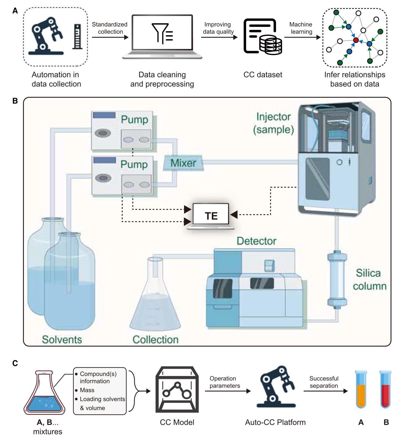
Figure 1. Schematic diagram of main parts
(A) Research pipeline (CC, column chromatography).
(B) Schematic of automation platform.
(C) Separation process schematic.
In order to address the aforementioned issue, our investigation focused on employing smaller format columns, such as 4 g columns, for data collection. These columns offer the advantages of reduced experimental time frames and lower solvent usage,
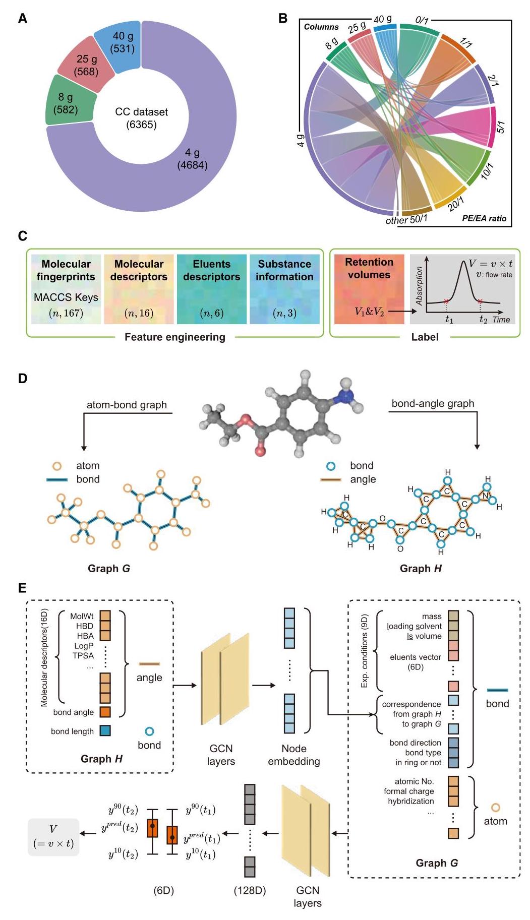
(legend on next page) which enables the rapid accumulation of a substantial dataset and facilitates the development of a foundational model. We successfully amassed a dataset comprising 4,684 standardized data points for 218 distinct compounds, spanning roughly 20 diverse compound classes, all analyzed using the 4 g columns. Detailed compound’s information can be found in Table S1. To enhance the generalizability of the experimental outcomes, each compound was subjected to testing across three distinct sample volumes and a range of seven eluent ratios at least. Moreover, we pursued selective data acquisition across columns with diverse specifications (Figure S2) and explored the application of transfer learning techniques to accommodate the variability in column characteristics; the forthcoming sections will delve into the specific applications and the effects of these methodologies with a detailed discussion.
Basic model with ML techniques
Following the completion of the data collection phase on the automated CC platform, we visualized the entire dataset, as depicted in Figures 2A and 2B. This visualization process clarified the structure of the dataset, which was compiled using four different specifications of chromatography columns, with data evenly distributed across the seven eluent ratios. For the reasons previously discussed, it was necessary to attempt the establishment of a basic model based on the $4\mathrm{\;g}$ dataset. Recognizing that the separation volume is a critical parameter in CC, we conducted an in-depth analysis of the UV spectral curves accurately determining it. This analysis allowed us to pinpoint the separation times for each compound $- {t}_{1}$ , marking the initial detection of the compound, and ${t}_{2}$ , indicating the moment when the compound was fully eluted out from the column. Figure 2C also gives a figurative definition of separation volume in this study, where ${V}_{1}$ and ${V}_{2}$ correspond to the volume of eluent consumed at the start of compound separation and at the time of complete elution, respectively. Thus, we have the following:
$$ {V}_{1} = v \times {t}_{1} $$(Equation 1)
$$ {V}_{2} = v \times {t}_{2}, $$(Equation 2)
$$ {\Delta V} = {V}_{2} - {V}_{1} = v \times \left( {{t}_{2} - {t}_{1}}\right) . $$(Equation 3)
Before constructing the ML model, appropriate feature engineering is needed to capture all the important factors that need to be considered in the experiment. Mechanistically, the main factors influencing the $V$ value are molecular polarity and experimental conditions. Molecular polarity is directly related to a compound’s structure and properties. The molecular access system (MACCS) keys are widely utilized structural keys that encapsulate information about the molecular structure, its fragments, and substructures. These keys allow for the transformation of any compound into a 167-dimensional representation. Additionally, the RDKit software facilitates the straightforward extraction of sixteen kinds of molecular properties (detailed in methods section), including total polar surface area (TPSA), molecular weight (MolWt), and the number of hydrogen bond donors (HBDs), etc. Moreover, there are several key parameters for CC experiments that need to be integrated, including the proportion of eluents, the type of loading eluent (e), compound mass (m), and the volume of loading eluent $\left( {V}_{e}\right)$ , converting these into algorithmic terms would result in a set of 9-dimensional experimental parameter features, consisting of 6-dimensional weighted descriptors for solvents and three-dimensional CC column information. In a systematic investigation to ascertain the predictive accuracy of diverse ML strategies, we scrutinized three distinct algorithms: light gradient boosting machine (LGB), artificial neural networks (ANNs), and graph neural networks (GNNs). Various algorithms handle parameters differently. For traditional algorithms such as LGB and ANN, parameters such as the feature engineering shown in Figure 2C are inputted directly into the training function without any special handling.
In our previous study, ${}^{14}$ we explored a geometry-enhanced GNN approach to molecular representation. This approach utilizes the natural graphical properties of molecular structures and integrates problem-relevant features into the graph representation. It combines the 3D conformation of the molecule, experimental conditions, relevant descriptors, and quantile learning techniques ${}^{17}$ to meet the specific needs of the chemical domain. The use of the quantile learning technique is essential to capture the uncertainty in the training process, providing a reasonable confidence interval for the predicted results. Additionally, combining expertise in mathematical modeling of chromatographic processes and column properties with ML algorithms further enhances the predictive accuracy of the models. This integrated approach has improved the efficiency and quality of data collection. It also provides a solid foundation for predictive modeling in CC. This is expected to lead to significant advances in the field of chemical analysis and purification.
Building on the foundation established by our geometry-enhanced GNN, this study further refines the application of GNNs in CC. The enhanced model not only maintains the integration of critical parameters but also leverages advanced algorithmic strategies to optimize the network structure. As illustrated in Figure 2D, the 3D conformation of a molecule can be divided into a graph G describing atom-bond and a graph H describing bond angle. Figure 2E provides a detailed illustration of the network architecture formation. The model’s feature input comprises 9-dimensional experimental parameter features and 16-dimensional molecular features, which are embedded into two distinct graph representations. In concrete terms, the 9-dimensional experimental parameter features are embedded
Figure 2. Dataset distribution and feature engineering
(A) Column specifications for number distribution.
(B) Distribution of the amount of data according to the proportion of eluents.
(C) Feature engineering for ANN and LGB.
(D) The schematic instruction of atom-bond graph G and bond-angle graph H.
(E) Schematic diagram of QGeoGNN hierarchy. into the edge features of graph G, representing experimental data. These edge features reflect the various proportions of eluents used in the chromatography experiments and other key experimental parameters, providing specific information about the experimental conditions to the model. Afterward, the 16-dimensional molecular features are embedded into the edge features of graph H. These molecular features, which include chemical and physical properties of the molecules, are crucial for capturing the interaction between molecules and silica particles, essential for predicting their behavior in CC. By utilizing graph isomorphism convolution (GIC) techniques, ${}^{18}$ the model effectively captures complex relationships and patterns between molecules and silica particles. This approach demonstrates superior performance compared with traditional methods, making it a valuable tool for predicting molecular behavior in CC. In the case of GNN, the column information is structured in a comparable manner and integrated into graph G. Further implementation details of these models are outlined in the methods section.
These models, each with inherent advantages and idiosyncrasies, were evaluated to furnish a holistic view of the efficacy of varied algorithms in processing chemical datasets. For this analysis, the dataset pertaining to CC was judiciously partitioned into three subsets: 80% was dedicated to the training set, with the remainder equally divided between validation and test sets (10% each). This stratagem was intended to allocate ample data for model training while reserving independent subsets for validation and testing, thereby facilitating a robust assessment of the models’ generalization capacities and empirical predictive prowess. The training set underpinned model learning and parameter optimization, the validation set served for model selection and hyperparameter refinement, and the test set was utilized for the ultimate evaluation of predictive performance. This methodological approach enabled a rigorous comparison of the performances of diverse ML algorithms on a uniform dataset, laying a scientific foundation for the selection of the most apt model for predicting outcomes in CC. Such a step is indispensable for guaranteeing the model’s reliability and precision, particularly when navigating the complexities inherent in chemical data analysis, where disparate ML models may demonstrate markedly different performance profiles.
The study’s model learning was based on data from a $4\mathrm{\;g}$ chromatography column, with the results shown in Figure 3A and Table 1. These results indicate that the LGB, a tree-based model, has somewhat limited predictive accuracy, with ${R}^{2}$ values for ${V}_{1}$ and ${V}_{2}$ being only around 0.69. While both ANN and QGeoGNN (quantum geometry-informed graph neural network) achieve comparable performance (with closely aligned ${R}^{2}$ values), their underlying mechanisms differ: ANN, as a general-purpose neural network, excels at processing structured data but may struggle to capture nuanced molecular interactions, whereas QGeoGNN integrates GNNs with molecular geometric features (e.g., conformations and stereochemistry) that critically influence chromatographic retention dynamics. Drawing from prior work in the HPLC domain, it is noted that QGeoGNN is capable of integrating both experimental parameters and molecular features effectively. Importantly, as the volume of data increases, the predictive performance of QGeoGNN shows an upward trend, which is crucial for handling large-scale chromatography data. Furthermore, it is observed that traditional GNN, which only include a single graph representation (graph G), perform relatively poorly in terms of ${R}^{2}$ . Based on the analysis and findings, the decision to utilize the QGeoGNN to construct a predictive model for CC is well founded. This choice is predicated on the advantages of QGeoGNN in handling complex chemical data, as well as its potential for enhanced performance in a big data environment. The implementation of QGeoGNN is expected to make the CC prediction model more promising, offering more accurate predictions for compound separation.
To comprehensively assess the performance of our developed predictive model, a series of tests were conducted. These tests were designed to reveal the model’s behavior under various conditions, including the relationship between compound structural similarity (tanimoto coefficient) and model prediction error (i.e., mean absolute error [MAE]), as well as the impact of training set proportion and noise ratio on model prediction accuracy $\left( {R}^{2}\right)$ . Initially, we explored the relationship between compound similarity and MAE through 20-fold cross-validation (Figure 3B). The results indicate that higher compound similarity corresponds to lower error in predicting separation volume, aligning with the general expectation that models predict chromatographic behavior more accurately when the structural similarity of compounds is high. Experimental data demonstrated that the ${R}^{2}$ value tends to stabilize when the training set proportion exceeds 50% and the noise ratio is maintained below 20% (Figures 3C and 3D). This suggests that under these conditions of dataset size and noise level, the model achieves robust predictive performance, indicating its resilience to training data quantity and noise. Furthermore, validation experiments were conducted to determine whether different compounds mixed together have the same retention volume as they do when in pure form. The experiments were performed on a few compounds that separated under specified conditions. The results (Figure S3) demonstrated that when the compounds have no interaction with each other and are within the appropriate mass range, their retention volume remains the same when mixed together as it does when they are in pure form.
Transfer learning
In the context of this study, 90% of our dataset comprises data from 4 g chromatography columns, resulting in a relatively homogeneous dataset and limited model generalization. However, in real experimental scenarios, chromatography columns come in various specifications. To address this, we implemented a transfer learning strategy, ${}^{{19} - {21}}$ enabling the model trained on $4\mathrm{\;g}$ data to be applicable to a wider range of column specifications, thereby enhancing its adaptability and performance across diverse datasets. The quintessence of transfer learning lies in its capacity to leverage knowledge acquired from one task to bolster learning efficiency and performance on another, closely related task. In this vein, specific segments of the extant model were meticulously adjusted to more aptly align with the requirements of the new dataset, thus epitomizing the strategic application of transfer learning principles in our research.
In the input layer of the model, we integrated information pertinent to new chromatographic column specifications (Figure 4A). This integration is a critical step as it enables the model to accommodate and process the unique characteristics of new chromatographic columns, ensuring the model’s ability to recognize and adapt to these novel operational conditions. The output layer of the model underwent updates to account for variations that different column specifications might introduce to the final results. Consequently, adjustments to the model’s final stages were necessary to accurately predict outputs for new specifications. This approach allows the model to adapt to new output requirements while retaining its existing knowledge base.
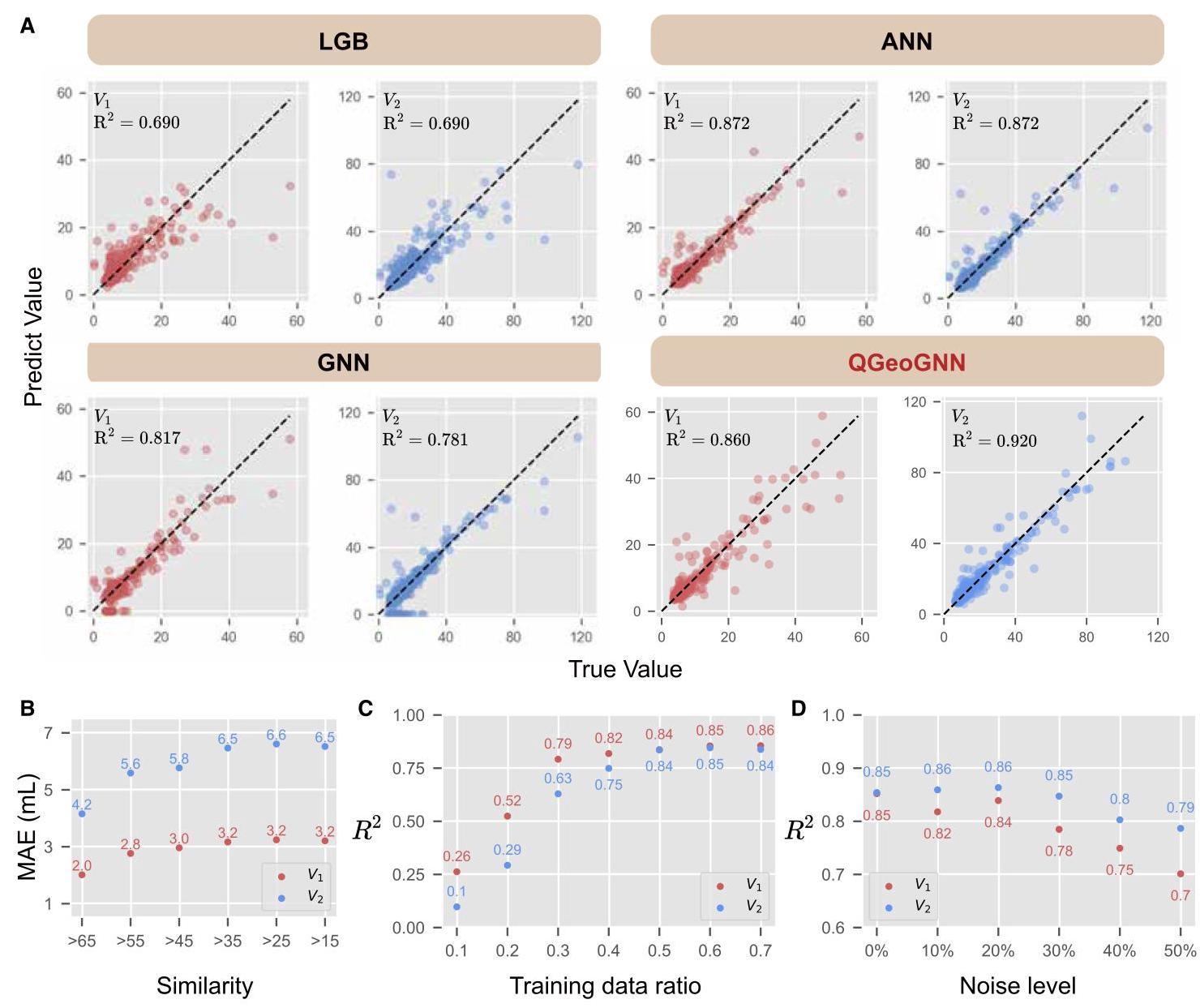
Figure 3. The training results of the basic model
(A) Training outcomes of different ML algorithms based on 4 g-dataset.
(B) Dependence of MAE on structural similarity (tanimoto coefficient).
(C) Impact of the training set proportion on ${R}^{2}$ .
(D) Influence of Gaussian noise ratio on ${R}^{2}$ .
Table 1. Quantitative metrics for $4\mathrm{\;g}$ base models using distinct algorithms
| Algo | ${R}^{2}\left( {V}_{1}\right) \uparrow$ | ${R}^{2}\left( {V}_{2}\right) \uparrow$ | MAE $\left( {V}_{1}\right) \downarrow$ | MAE $\left( {V}_{2}\right) \downarrow$ | RMSE $\left( {V}_{1}\right) \downarrow$ | RMSE $\left( {V}_{2}\right) \downarrow$ |
| LGB | 0.690 | 0.690 | 1.792 | 3.504 | 3.307 | 5.991 |
| ANN | 0.872 | 0.872 | 1.381 | 2.218 | 2.512 | 4.483 |
| GNN | 0.817 | 0.781 | 1.744 | 3.322 | 2.901 | 6.303 |
| QGeoGNN | 0.859 | 0.913 | 1.452 | 2.475 | 2.649 | 4.235 |
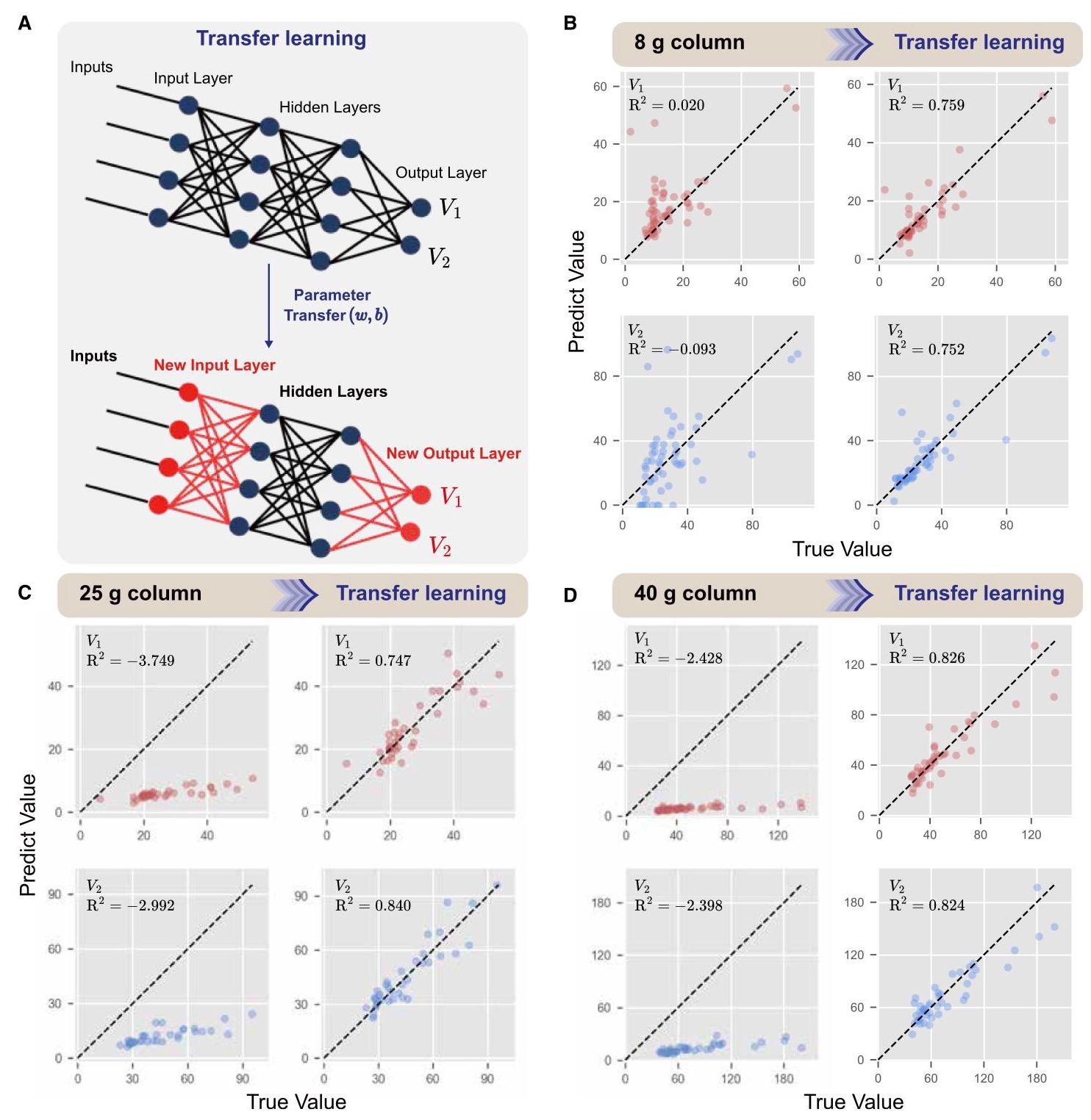
Figure 4. Transfer learning and training results
(A) Transfer learning process.
(B-D) Training results from the application of transfer learning to the 8, 25, and 40 g column datasets using the QGeoGNN model initially developed for the 4 g.
During the application of transfer learning, we opted for a strategy that involved transferring the parameters of the original network to a new network and adopted a lower learning rate $\left( {10}^{-4}\right)$ during the training part. Compared with the data volume for the $4\mathrm{\;g}$ column, these smaller-scale tasks could lead to over-fitting ${}^{{22},{23}}$ when training complex models like QGeoGNN from scratch. This decision was primarily based on the following considerations: due to the limited amount of data, it is crucial to avoid overfitting. ${}^{24}$ To achieve this, we employed a pre-trained model and applied a lower learning rate to fine-tune it, thus ensuring more stable and generalized performance. ${}^{25}$ Additionally, we leveraged features learned from the $4\mathrm{\;g}$ base model,
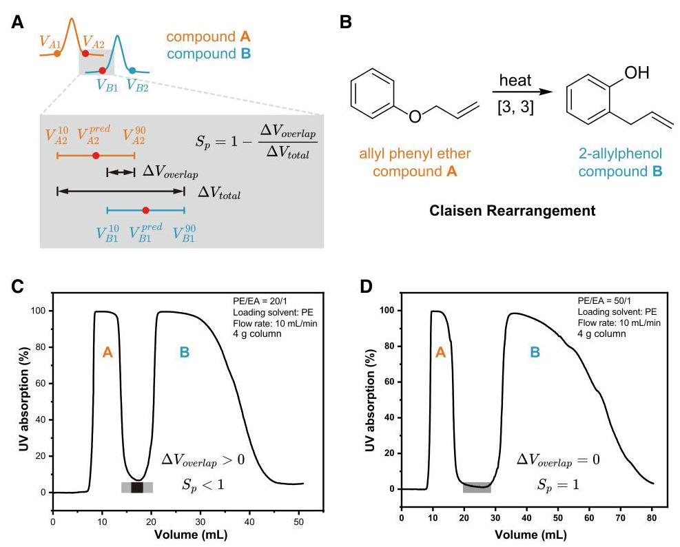
Figure 5. Application of ${S}_{p}$ in CC predictive model
(A) Schematic diagram of ${S}_{p}$ calculation. (B) The classic Claisen rearrangement reaction. (C and D) Wet laboratory validation based on model prediction results. such as 3D molecular information, to expedite training and conserve computational resources and time for the new models. ${}^{26}$ By gradually adjusting the model weights, we can more effectively balance the knowledge between the new and the old datasets, thereby enhancing the model’s generalization performance in new chromatographic column specifications.
Operationally, we selected the basic model with the minimum MAE on the $4\mathrm{\;g}$ column, updated its output layer, and fine-tuned these parts using parameters from the new tasks. The application of transfer learning methods to chromatography column datasets of different specifications (8, 25, and 40 g) and the comparison of their effectiveness against direct training methods reveal significant insights. Specifically, for the $8\mathrm{\;g}$ column (Figure 4B), we initially employed the same direct training approach used for the $4\mathrm{\;g}$ column. However, this approach yielded lower prediction accuracy, with ${R}^{2}$ values for ${V}_{1}$ and ${V}_{2}$ being only 0.02 and -0.093 , respectively. This outcome indicates that the direct training method is not sufficiently effective when dealing with new chromatography column specifications. In contrast, the application of the transfer learning method resulted in a significant improvement in the model’s predictive capabilities. Specifically, on the $8\mathrm{\;g}$ chromatography column dataset, the model adjusted through transfer learning achieved ${R}^{2}$ values of 0.759 and 0.752 for ${V}_{1}$ and ${V}_{2}$ , respectively. Similarly, we observed a comparable trend in datasets for the 25 and 40 g chromatography columns (Figures 4C and 4D). Furthermore, we investigated the potential for extending the dichloromethane/methanol (DCM/MeOH) eluent system and conducted additional experiments on bonded columns. We discovered that transfer learning improved performance in both scenarios, with the ${R}^{2}$ values increasing from approximately 0 to nearly 0.6 (Figure S4). This substantial improvement not only validates the effectiveness of transfer learning in enhancing model predictive capability but also highlights its suitability for handling data from chromatography columns of varying specifications and eluent systems.
Application: Separation probability
To quantitatively assess the separation probability $\left( {S}_{p}\right)$ of compounds under specific conditions, we introduced an ${S}_{p}$ formula based on confidence interval. This formula calculates the ${S}_{p}$ based on the quantiles of elution volumes $\left( V\right)$ of two compounds during the chromatographic process. The calculation method for the ${S}_{p}$ involves specific quantile-based measurements. We define the 90th percentile of the ${V}_{2}$ of the compound $\mathbf{A}$ as ${V}_{A2}^{90}$ and the 10th percentile of the ${V}_{1}$ of the compound $\mathbf{B}$ as ${V}_{B1}^{10}$ . Similarly, the 90th percentile of the ${V}_{1}$ of the compound $\mathbf{B}$ is ${V}_{B1}^{90}$ , and the 10th percentile of the ${V}_{2}$ of the compound $\mathbf{A}$ is ${V}_{A2}^{10}$ .
As depicted in Figure 5A, assuming that compound $\mathbf{A}$ be eluted out first, the ${S}_{p}$ is then derived based on these quantile values:
$$ {S}_{p} = 1 - \frac{\max \left( {0,{V}_{A2}^{90} - {V}_{B1}^{10}}\right) }{{V}_{B1}^{90} - {V}_{A2}^{10}}. $$(Equation 4)
The logic of this formula is based on the overlap of the elution times of the two compounds in chromatography column. If the value of $\left( {{V}_{A2}^{90} - {V}_{B1}^{10}}\right)$ is positive, it suggests that ${V}_{B1}$ could be less than ${V}_{A2}$ , indicating that the separation of the two compounds may not be fully achieved. If the value is negative, it indicates complete separation of the two compounds, with an ${S}_{p}$ close to 1.
To provide a more concrete and visual explanation of ${S}_{p}$ and to demonstrate its practical application in real experiments, we selected a classic chemical reaction, the Claisen reaction, ${}^{27}$ as the experimental subject (Figure 5B). Due to the reversibility of this reaction, both reactants and products coexist in the post-reaction mixture, making the separation of high-purity products essential. Initially, we utilized the predictive model to determine the parameters required for effective separation. In order to facilitate the procedure, pure allylphenyl ester (compound A) and 2-allylphenol (compound B) are combined directly in a 1:1 ratio as an alternative to the reaction mixture. Subsequently, an adequate quantity of the up-sampling solvent was introduced to satisfy the minimum sample volume requirement of the injector. Subsequently, the experiment was initiated at the control terminal, yielding the corresponding experimental results as shown in Figures 5C and 5D. The corresponding ${S}_{p}$ is obtained by quantile calculation, when petroleum ether (PE)/ethyl acetate (EA) $= {20}/1$ , the predicted value of ${S}_{p}$ is 0.51 . It is clear that there is indeed some intersection in the separation process of A and B, which means that they are not completely separate. Also, when PE/EA = 50/1, the predicted value of ${S}_{p}$ is 1.0, there is no intersection in the separation process of A and B, which means that they are completely separated. This validation result demonstrates the practical value of ${S}_{p}$ in guiding the separation of actual products. Using the Claisen reaction as an example, our model accurately predicted outcomes under different experimental conditions. Detailed prediction data can be found in Table S2.
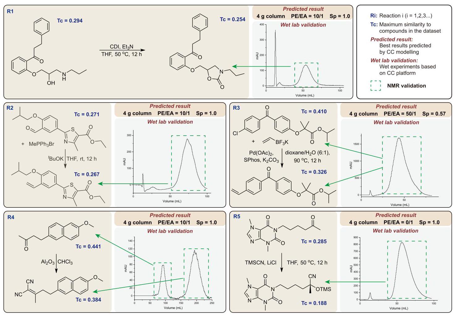
Figure 6. Prediction and validation of ${S}_{p}$ for complex compound reactions
As previously demonstrated, the model exhibits satisfactory prediction accuracy within the dataset. However, this alone is insufficient to address the complexities of CC comprehensively. A more critical aspect is the model’s ability to predict ${S}_{p}$ values for separating compounds outside the dataset. To evaluate this, we selected several products of classical organic reactions (Figure S5A) for experimental validation. The model demonstrated 90% accuracy in predicting separation outcomes ( ${S}_{p}$ values) across 70 experimental validation points from 10 compound groups, successfully correlating PE/EA solvent ratio effects with experimental results (Figures S5B and S5C). This demonstrates that the ${S}_{p}$ values generated by our CC prediction model provide reliable guidance for compound separation processes.
While the examples based on classic name reactions may appear basic, they effectively establish the model’s feasibility for large-scale application beyond the dataset. To further assess the model’s performance in complex compound reactions, we performed CC separations on mixtures from five distinct reactions under model-predicted optimal conditions (Figure 6). For reactions R1 and R2, where substrates were more polar than their respective products, the products eluted first as anticipated. Subsequent NMR analysis confirmed the high purity of these isolated products. Reaction R3 demonstrated limited separation potential due to negligible polarity differences between substrate and product, which was corroborated by NMR showing inseparable components. In R4, the predicted elution sequence (substrate followed by product) was validated through two distinct UV absorption peaks, with NMR confirming peak assignments. For the highly polar system in R5, exclusive use of pure EA as eluent successfully yielded high-purity product as predicted, with NMR verification. Complete NMR spectra are provided in the appendix in Document S1.
Moreover, the predictive models obtained through transfer learning (8, 25, and 40 g models, with three sets of experiments each) were further validated to demonstrate their generalization guidance capability. The results (Figures S6-S8) demonstrated that the parameters predicted by these models could effectively optimize the compound separation process under different chromatographic column specifications. Current CC prediction models rely on UV detection, but there are compounds with weak or no UV absorption. To address this, we selected a set of compounds labeled L and M (Figure S9). Compound L has no UV absorption, whereas compound M does. Their SMILES were input into the prediction model to obtain separation conditions, which were then tested on the CC experimental platform. TLC results were clear, showing distinct spots for both compounds. Compound L, without UV absorption, appeared in tube 3, and compound M, with UV absorption, was found in tubes 12 and 13. These results demonstrate that the CC prediction model can predict separation conditions regardless of UV absorption, though there is potential for improving detection methods. The validation results confirm that our model can successfully predict the ${S}_{p}$ of complex mixtures, validating its effectiveness and robustness.
DISCUSSION
This study developed ML models tailored for CC to address the challenges of inaccuracy and reproducibility in traditional empirical workflows. An automated chromatography platform enabled standardized data acquisition, while the QGeoGNN algorithm - incorporating molecular 3D conformations, experimental parameters, and domain-specific descriptors - was optimized through transfer learning for diverse column specifications. A novel ${S}_{p}$ metric was established to guide experimental design, with validation confirming the baseline and transfer learning-adapted models effectively predict retention volumes. Critically, the model focuses on predicting retention behavior for known components (e.g., reactants, products, and pre-characterized byproducts) under controlled separation scenarios, offering a mechanism-driven pathway to reduce empirical optimization efforts in deterministic systems.
The model’s scope and validation logic align with its theoretical framework. While chromatographic separation inherently depends on structural information-limiting its utility for unknown impurities - the approach demonstrates universal applicability to any characterized compounds. Challenges in separating unidentified components stem from the technology’s intrinsic constraints, not the model itself. For systems with speculatively identifiable species, the framework provides actionable elution prediction schemes, as validated in raw material-product separation cases.
Nevertheless, limitations persist. The dataset’s compound diversity remains constrained, and the current eluent system (PE/ EA) prioritizes less polar compounds, though transfer learning extends applicability to DCM/MeOH. Other systems (e.g., MeOH/TCM) require further data integration. Additionally, ${S}_{p}$ -defined based on empirical chromatography principles-does not yet incorporate factors such as column temperature or stationary phase effects. Future work will explore these variables and expand community-driven validation through open-source model iterations to enhance adaptability across broader chemical scenarios.
METHODS
Construction and control of automation equipment
To address the challenges encountered in CC experiments, we have designed and assembled an advanced automated apparatus specifically for the collection of CC data. The construction and operational principle of the device are depicted in Figure 1B (a photograph of the apparatus is provided in Figure S1). The system incorporates two medium-pressure pumps (manufactured by Beijing Qingbohua Technology), each delivering different pure solvents (PE and EA) with a flow accuracy of ${0.01}\mathrm{{mL}}/\mathrm{{min}}$ and a maximum flow capacity of ${200}\mathrm{\;{mL}}/\mathrm{{min}}$ . To facilitate the mixing of eluents in multiple proportions, the outlets of these pumps are connected to a mixer, ensuring that the mobile phase can be thoroughly mixed in predetermined ratios before the elution step. The centerpiece of the system is an autosampler, which stores and automatically transports the prepared sample solutions, activating automatically upon receiving programmed instructions. Real-time signals during the separation process are captured and recorded by an ultraviolet detector operating at a wavelength of 254 nm. For real-time response and data synchronization, the pumps, detector, and autosampler are all connected via RS232 serial ports for real-time communication. Control over the entire automated platform is executed through a Python program, which manages sample positioning, flow rate adjustments, eluent proportioning, and the collection, conversion, analysis, and archiving of real-time detection signals. A video of the experiment is provided in the supplemental information (Data S2).
Construction of the CC dataset
In this study, a CC dataset comprising separation volume data for 218 compounds was collected using an automated experimental platform. The dataset encompasses 6,365 records of separation volumes, along with experimental conditions and column information. The dataset utilized for pre-training the basic model consists of 4,684 entries of 218 compounds, employing columns of $4\mathrm{\;g}$ specifications and includes comparisons of two different flow rates. The datasets for transfer learning correspond to different column specifications, with 582 data points of 90 compounds using 8 g columns, 568 data points of 80 compounds using 25 g columns, and 531 data points of 81 compounds using ${40}\mathrm{\;g}$ columns. Notably, the compounds for different columns are all within the scope of the 218 compounds, with detailed distributions available in the supplemental methods.
Flow rates were set based on the manufacturer’s recommendations: ${10}\mathrm{\;{mL}}/\mathrm{{min}}$ for a $4\mathrm{\;g}$ column, ${10}\mathrm{\;{mL}}/\mathrm{{min}}$ for an $8\mathrm{\;g}$ column consisting of two $4\mathrm{\;g}$ columns connected in series, ${15}\mathrm{\;{mL}}/\mathrm{{min}}$ for a 25 g column, and ${30}\mathrm{\;{mL}}/\mathrm{{min}}$ for a ${40}\mathrm{\;g}$ column. These settings were found to be reasonable and efficient during pre-tests, resulting in high-quality data collection. The photos of the chromatographic columns are also displayed in Figure S3. It took 6 months to collect the data, using approximately 600 L of PE, 180 L of EA, and 20 L of DCM). The DCM is utilized to load samples and clean the injection syringe.
All data indices are compiled in a comma-separated values (CSV) spreadsheet, where compounds are indexed by their Chemical Abstracts Service (CAS) numbers, and column specifications are differentiated in the column specification field. Recorded variables include flow rate, eluent ratio, compound purity, compound density, sample loading mass/volume, solvent volume for sample loading, with the “ending time” denoting the name of the UV original data. These identifiers are used to index corresponding data for subsequent analysis. Upon analysis completion, two columns, ${t}_{1}$ and ${t}_{2}$ , are generated, representing the start and end times of separation, respectively. A value of -1 for ${t}_{1}$ and ${t}_{2}$ indicates invalid data. The SMILES descriptors for compounds are generated using a Python script that converts molecular names into SMILES notation.
The graph representation for molecules
In this study, molecular representation was achieved by constructing two graphs, graph G and graph H, as illustrated in Figure 2D. Graphs are frequently employed in data science to depict unstructured data such as social networks, chemical molecules, and transportation networks. A typical graph consists of multiple nodes and edges that represent the connection relationships between them. ${}^{14}$ As shown in Figure 2E; graph G represents the planar structure of a chemical molecule, with nodes corresponding to atoms and edges representing chemical bonds. Each node in graph G encompasses nine attributes of the corresponding atom, including atomic number, chiral tag, degree, explicit valence, formal charge, hybridization, implicit valence, aromaticity, and the number of connected hydrogen atoms. The features of each edge in graph G include three properties of the bond and four experimental condition attributes; the bond properties comprise bond direction, bond type, and whether it is part of a ring, while the four experimental condition attributes include eluent ratio, sample mass, type of sample solvent, and mass of sample solvent.
Graph H encodes the quantum-geometric relationships by representing the 3D molecular conformation. The 3D conformation generation protocol is as follows: the process begins with RDKit’s ETKDGv3 algorithm, which performs stochastic conformer sampling to generate an initial ensemble of molecular conformations. Subsequently, these sampled conformers undergo molecular mechanics optimization using the MMFF94 force field, incorporating default partial charge assignments to refine their energy profiles. Finally, the lowest-energy conformer from the optimized set is systematically selected and utilized as the geometric input for the QGeoGNN framework, ensuring energy-minimized and physically plausible molecular representations for downstream computations. In this graph, nodes represent bond vectors and edges encode angular relationships between bonds. Each node in graph $H$ contains the length of the corresponding bond, while edges feature 17 geometric-chemical descriptors: the bond angle complemented by 16 quantum chemically relevant features including MolWt, HBDs, hydrogen bond acceptors (HBAs), octanol/water partition coefficient (LogP), TPSA, and 11 Mordred-calculated descriptors (Table S3). The core mechanism for integrating global molecular features is detailed in the supplemental methods. These descriptors were selected based on Spearman correlation analysis with separation time measurements.
Strategies for transfer learning
To elucidate the generality and adaptability of our model across various chemical datasets, the current research adopts a strategy of transfer learning. In the regime of transfer learning, the model is primed with weights acquired from antecedent training endeavors. This approach is eminently suited for contexts with constrained data availability or inherent similarities across tasks, thereby augmenting the model’s proficiency in assimilating data from novel domains. Training of the model engaged the mean-squared error (MSE) as the criterion for loss, appraising the divergence between predicted outcomes and actual observations. A learning rate scheduler (StepLR) was employed to dynamically modulate the learning rate, enhancing the training protocol, with the ultimate learning rate established at 0.0001 . Through relentless performance evaluations on the validation dataset, the generalization capacity of the model was meticulously monitored, culminating in a definitive performance appraisal on the test dataset to validate the model’s effectiveness and precision.
Experimental verification
In this study, several similarity thresholds are utilized to differentiate the similarity level including 65%, 55%, 45%, 35%, 25%, and 15%. Therefore, all data are categorized into six groups where the molecules in each group as the testing dataset have at least one similar molecule in the training dataset above a specific similarity (tanimoto similarity) threshold. Our objective was to assess the impact of training set size and data noise ratio on the performance of ML models. The noise follows a uniform distribution and is proportionally scaled to the original data. To systematically investigate the effects, we varied the proportions of the training set and the noise ratios. The training set proportions were set at 0.1, 0.2, 0.3, 0.4, 0.5, 0.6 , and 0.7 , while the noise ratios were adjusted to 0%, 10%, 20%, 30%, 40%, and 50%. Through this approach, we explored the robustness and generalization capabilities of the model when faced with varying degrees of data noise and different magnitudes of training data. Data preprocessing, including cleaning, normalization, and feature selection, was undertaken to ensure data quality. The dataset was partitioned according to the specified proportions of the training set to evaluate the influence of different volumes of training data on model performance. In each experiment, a certain proportion of the data was reserved as a test set to assess the model’s generalization ability.
Derivation of chromatographic ${S}_{p}$
In this work, we have defined a measurement method termed as chromatographic ${S}_{p}$ to quantify the likelihood of a ML model correctly separating the mixture of compounds under specific experimental conditions. This section elaborates on the definition and derivation of chromatographic ${S}_{p}$ . Utilizing the proposed QGeoGNN, we can ascertain the range of separated volume for the compounds. The definition of ${S}_{p}$ is grounded on a straightforward principle: regions within the numerical range overlap are deemed inseparable, whereas others are considered separable. Thus, ${S}_{p}$ can be articulated as Equation 4. This represents one specific scenario and does not encompass all computational approaches. Furthermore, the framework extends beyond binary separations to multicomponent systems.
For two-component separation, the probability is defined as the following:
Experimental settings and parameters
In the QGeoGNN utilized in this work, the number of GINConv is 5, the graph pooling strategy is the summation, the embedding dimension of the node and edge representation is 128 , and the batch size is 2,048. The training epoch is 1,500, and the validate loss is adapted for early stopping. For pre-train prediction, the prediction models are established for $4\mathrm{\;g}$ columns. The optimizer is Adam, and the learning rate is 0.001 . The subdataset is randomly divided into 80/10/10 to obtain the training, validating, and testing dataset. For comparison, the LGB, ANN, and GNN are also employed to train a predictive model. The input of LGB and ANN is composed of the 167-dimensional MACCS keys that are utilized to represent the molecular structure, the 16-dimensional molecular descriptors that are the same as those
$$ {P}_{i, j} = \left\{ \begin{array}{ll} {1.0} & \text{ if }{V}_{i}^{{10}\% } - {V}_{i}^{{90}\% } > 0 \\ 1 - \frac{\max \left( {0,\min \left( {{V}_{i}^{{90}\% },{V}_{i}^{{90}\% }}\right) - \max \left( {{V}_{i}^{{10}\% },{V}_{i}^{{10}\% }}\right) }\right) }{\max \left( {{V}_{i}^{{90}\% },{V}_{i}^{{90}\% }}\right) - \min \left( {{V}_{i}^{{10}\% },{V}_{i}^{{10}\% }}\right) } & \text{ otherwise } \end{array}\right. $$(Equation 5)
where ${V}_{i}^{{10}\% },{V}_{i}^{{50}\% },{V}_{i}^{{90}\% }$ represent the ${V}_{1}^{{10}\% },{V}_{1}^{{50}\% }$ , and ${V}_{1}^{{90}\% }$ values of compound $i$ .
The elution order is determined by ${V}_{i}^{{50}\% } \leq {V}_{i}^{{50}\% }$ , with the formula implicitly incorporating the sorting process.
Complete separation: occurs when ${V}_{j}^{{10}\% } > {V}_{i}^{{90}\% }$ .
Overlap scenario:
Numerator: overlap length (max(0, overlapend - overlapstart)).
Denominator: total span of both elution windows.
Separation degree: ${S}_{p} = 1 - \frac{\text{ overlap }}{\text{ total span }}$ .
For multicomponent systems $\left( {n \geq 3}\right)$ , the ${S}_{p}$ generalizes to the following:
$$ {S}_{p} = \mathop{\prod }\limits_{{1 \leq i < j \leq n}}{P}_{i, j} $$(Equation 6)
where $n$ is the total number of compounds.
The product iterates over all unique pairwise combinations (e. g., ${S}_{p} = {P}_{1,2} \times {P}_{1,3} \times {P}_{2,3}$ for three compounds).
Practical implications:
The combined formulas enable prediction of ${S}_{p}$ under varying eluent ratios (fixed column specifications and flow rate).
For mixtures with $n \geq 3$ , secondary analysis may identify compounds with ${P}_{ij} = 1$ against others, allowing prioritized isolation under optimized conditions before separating remaining components.
Hence, the defined chromatographic ${S}_{p}$ spans from 0 to 1 . A higher ${S}_{p}$ value indicates an expanded region of separability, in other words, an increased likelihood that the mixture of compounds is predicted to be separable by the QGeoGNN. utilized in QGeoGNN, and 9-dimensional experimental parameter features. For LGB, the maximum depth is 5, the learning rate is 0.007 , the number of leaves is 25 , and the number of estimators is 1,000. For ANN, there are 3 hidden layers with 50 hidden neurons in each hidden layer. The activation function is leaky ReLu and the optimizer is Adam with a learning rate of 0.001 . The training epoch is 10,000 and early stopping is adopted. The construction of GNN is similar to QGeoGNN, while it only has graph G, and the loss function is of the MSE between the predicted and observed value. The experimental parameter features are incorporated into the edge features for GNN. For transfer learning, the individual secondary datasets are split into ${80}/{10}/{10}$ to train a transfer model.
RESOURCE AVAILABILITY
Lead contact
Requests for further information and resources should be directed to and will be fulfilled by the lead contact, Fanyang Mo ().
Materials availability
This study did not generate new unique reagents.
Data and code availability
The CC dataset generated in this study has been deposited in a GitHub repository: https://github.com/danielwu0415/column_chromatography_prediction/ tree/main/dataset. Source data are provided with this paper. All original code can be found in a GitHub repository: https://github.com/danielwu0415/ column_chromatography_prediction/tree/main/application.
ACKNOWLEDGMENTS
This work is supported by the Natural Science Foundation of China (grant nos. 22071004, 21933001, and 22150013, received by F.M.). F.M. thanks the
Peking University Shenzhen Graduate School and the Shenzhen Government for the start-up funding support. We thank the High-Performance Computing Platform of Peking University for ML model training. We also extend our gratitude to all the reviewers for their insightful and constructive feedback, which has greatly contributed to the enhancement of our work.
AUTHOR CONTRIBUTIONS
W.W. and F.M. established the automated platform. W.W. conducted experiments and collected the CC dataset. W.W. and H.X. analyzed the data. W.W. and H.X. performed chemoinformatic and ML studies. Yang Xu, Q.Z., and Yan Xu conducted organic reactions. P.L. conducted the ${}^{1}\mathrm{H}$ NMR analysis. Y.C. contributed to algorithmic discussions and provided feedback on framework design. W.W. and F.M. wrote the manuscript with the discussion feedback from all authors. F.M. conceived the idea and designed the overall research. F.M. supervised the whole project.
DECLARATION OF INTERESTS
F.M., W.W., H.X., and D.Z. are inventors on a patent application (CN 202410282149.7) submitted by Peking University that covers an ML method for CC conditions prediction.
SUPPLEMENTAL INFORMATION
Supplemental information can be found online at https://doi.org/10.1016/j.chempr.2025.102598.
Received: October 31, 2024
Revised: March 24, 2025
Accepted: April 28, 2025
Published: May 29, 2025
REFERENCES
Still, W.C., Kahn, M., and Mitra, A. (1978). Rapid chromatographic technique for preparative separations with moderate resolution. J. Org. Chem. 43, 2923-2925.
Stocker, S., Csányi, G., Reuter, K., and Margraf, J.T. (2020). Machine learning in chemical reaction space. Nat. Commun. 11, 5505. https:// doi.org/10.1038/s41467-020-19267-x.
Keith, J.A., Vassilev-Galindo, V., Cheng, B., Chmiela, S., Gastegger, M., Müller, K.R., and Tkatchenko, A. (2021). Combining machine learning and computational chemistry for predictive insights into chemical systems. Chem. Rev. 121, 9816-9872. https://doi.org/10.1021/acs.chem-rev.1c00107.
Meuwly, M. (2021). Machine learning for chemical reactions. Chem. Rev. 121, 10218-10239. https://doi.org/10.1021/acs.chemrev.1c00033.
Jumper, J., Evans, R., Pritzel, A., Green, T., Figurnov, M., Ronneberger, O., Tunyasuvunakool, K., Bates, R., Zídek, A., Potapenko, A., et al. (2021). Highly accurate protein structure prediction with alphafold. Nature 596, 583-589. https://doi.org/10.1038/s41586-021-03819-2.
Hudson, D., Fernandes, R.A., Basham, M., Ogg, G., and Koohy, H. (2023). Can we predict t cell specificity with digital biology and machine learning? Nat. Rev. Immunol. 23, 511-521. https://doi.org/10.1038/s41577-023- 00835-3.
Kaissis, G.A., Makowski, M.R., Rückert, D., and Braren, R.F. (2020). Secure, privacy-preserving and federated machine learning in medical imaging. Nat. Mach. Intell. 2, 305-311.
Varoquaux, G., and Cheplygina, V. (2022). Machine learning for medical imaging: methodological failures and recommendations for the future. npj Digit. Med. 5, 48. https://doi.org/10.1038/s41746-022-00592-y.
Manzano, J.S., Hou, W., Zalesskiy, S.S., Frei, P., Wang, H., Kitson, P.J., and Cronin, L. (2022). An autonomous portable platform for universal chemical synthesis. Nat. Chem. 14, 1311-1318. https://doi.org/10.1038/ s41557-022-01016-w.
Zhu, Q., Huang, Y., Zhou, D., Zhao, L., Guo, L., Yang, R., Sun, Z., Luo, M., Zhang, F., Xiao, H., et al. (2023). Automated synthesis of oxygen-producing catalysts from martian meteorites by a robotic ai chemist. Natl. Synth. 3, 319-328.
Li, S.W., Xu, L.C., Zhang, C., Zhang, S.Q., and Hong, X. (2023). Reaction performance prediction with an extrapolative and interpretable graph model based on chemical knowledge. Nat. Commun. 14, 3569. https:// doi.org/10.1038/s41467-023-39283-x.
Xu, H., Lin, J., Liu, Q., Chen, Y., Zhang, J., Yang, Y., Young, M.C., Xu, Y., Zhang, D., and Mo, F. (2022). High-throughput discovery of chemical structure-polarity relationships combining automation and machine-learning techniques. Chem 8, 3202-3214.
Xu, H., Zhang, D., and Mo, F. (2022). High-throughput automated platform for thin layer chromatography analysis. Star Protoc. 3, 101893. https://doi.org/10.1016/j.xpro.2022.101893.
Xu, H., Lin, J., Zhang, D., and Mo, F. (2023). Retention time prediction for chromatographic enantioseparation by quantile geometry-enhanced graph neural network. Nat. Commun. 14, 3095. https://doi.org/10.1038/ s41467-023-38853-3.
Filipa de Almeida, A., and Rodrigues, T. (2023). Machine Learning for the Optimization of Chemical Reaction Conditions (Wiley Online Library).
Burés, J., and Larrosa, I. (2023). Organic reaction mechanism classification using machine learning. Nature 613, 689-695. https://doi.org/10.1038/s41586-022-05639-4.
Zhang, W., Quan, H., and Srinivasan, D. (2018). An improved quantile regression neural network for probabilistic load forecasting. IEEE Trans. Smart Grid 10, 4425-4434.
Xu, K., Hu, W., Leskovec, J., and Jegelka, S. (2019). How Powerful Are Graph Neural Networks?. Preprint at arXiv. https://doi.org/10.48550/arXiv.1810.00826.
Yang, L., Hanneke, S., and Carbonell, J. (2013). A theory of transfer learning with applications to active learning. Mach. Learn. 90, 161-189.
Zhuang, F., Qi, Z., Duan, K., Xi, D., Zhu, Y., Zhu, H., Xiong, H., and He, Q. (2020). A comprehensive survey on transfer learning. Proc. IEEE 109, 43-76.
Niu, S., Liu, Y., Wang, J., and Song, H. (2020). A decade survey of transfer learning (2010-2020). IEEE Trans. Artif. Intell. 1, 151-166.
Rice, L., Wong, E., and Kolter, J.Z. (2020). Overfitting in Adversarially Robust Deep Learning. Preprint at arXiv. https://doi.org/10.48550/arXiv.2002.11569.
Salman, S., and Liu, X. (2019). Overfitting Mechanism and Avoidance in Deep Neural Networks. Preprint at arXiv. https://doi.org/10.48550/arXiv.1901.06566.
Park, M.J., and Sacchi, M.D. (2020). Automatic velocity analysis using convolutional neural network and transfer learning. Geophysics 85, V33-V43.
Huang, Y., Liang, Y., and Huang, L. (2022). Provable generalization of overparameterized meta-learning trained with sgd. NeurIPS 35, 16563- 16576.
Shao, S., McAleer, S., Yan, R., and Baldi, P. (2018). Highly accurate machine fault diagnosis using deep transfer learning. IEEE Trans. Ind. Inform. 15, 2446-2455.
Martín Castro, A.M. (2004). Claisen rearrangement over the past nine decades. Chem. Rev. 104, 2939-3002. https://doi.org/10.1021/cr020703u.