Thermodynamic analysis of a novel multi-target temperature transcritical CO2 ejector-expansion refrigeration cycle with vapor-injection
中文 / Bilingual · English version
Min-Qiang Zeng ${}^{a}$ , Qiu-Yun Zheng ${}^{c}$ , Xue-Lai Zhang ${}^{a}$ , Fan-Yang Mo ${}^{b}$ , Xin-Rong Zhang ${}^{b, c, * }$
a Merchant Marine College, Shanghai Maritime University, Shanghai, 201306, China
${}^{\mathrm{b}}$ Department of Energy and Resources Engineering, College of Engineering, Peking University, Beijing,100871, China
c Beijing Engineering Research Center of City Heat, Beijing, 100871, China
A R T I C L E I N F O
Keywords:
Transcritical ${\mathrm{{CO}}}_{2}$ cycle
Ejector
Vapor-injection
Multi-target temperature
A B S T R A C T
In the present paper, a multi-target temperature ejector-expansion subcooler vapor-injection refrigeration cycle is proposed in order to improve the performance of natural fluid ${\mathrm{{CO}}}_{2}$ refrigeration cycles. A thermodynamics model to simulate a two-phase ejector cycle integrating a vapor-injection is first established from the energetic and exergetic perspectives. The behavior of the new cycle is then analyzed, and the adjustment direction of the cooling capacity and the evaporating temperature is pointed out. Furthermore, the new cycle is also compared with the subcooler vapor-injection refrigeration cycle and the ejector-expansion refrigeration cycle. The obtained results show that the behavior of the evaporators is affected by the bypass mass ratio and the entrainment ratio, and the two parameter determines the direction of adjusting the cooling capacity distribution and the evaporating temperature. The COP of the new cycle is about 17.9-29.4% and 2.8-7.8% higher than that of subcooler vapor-injection refrigeration cycle and ejector-expansion refrigeration cycle; the exergy efficiency of new cycle is about 14-28.2% and 3.7-11.3% higher than that of subcooler vapor-injection refrigeration cycle and ejector-expansion refrigeration cycle; and it is also found that the performance of the new cycle is improved more significantly under low cooling temperature and high ambient temperature conditions.
1. Introduction
With the development of cold chain logistics and the increasing demand for food refrigeration and freezing, so far, nearly 20% of the electricity consumed worldwide is used for refrigeration and the demand for refrigerating is expected to grow tenfold by 2050 [1,2]. The critical impact of the refrigeration industry on ozone depletion and global warming has developed into an alarming issue, which is mainly because of the wide application of HCFCs and HFCs refrigerants [3], which are intended to be gradually replaced by more sustainable alternatives. On October 15, 2016, the Kigali Amendment to the Montreal Protocol reached an agreement on the reduction of HFCs and pointed out that HFCs’ production and consumption are to be phased down gradually by between 80 and 85% from 2019 to the late 2040s [4].
To alleviate the increasingly serious environmental problems around the world, finding and developing green renewable energy sources and improving energy efficiency are urgent issues in the refrigeration field [5], natural refrigerants (such as ${\mathrm{{CO}}}_{2},{\mathrm{{NH}}}_{3},\mathrm{R}{290}$ , etc.) are gradually becoming one of its solutions. Although proper performance can be obtained by using R717, its adoption is not widespread due to its toxicity [6]. HCs (R290, R600a, R1270, etc.) safety is the main bottleneck restricting large-scale applications [7]. ${\mathrm{{CO}}}_{2}$ is considered to be a very potentially environmentally friendly alternative refrigerant due to its good thermophysical properties [8-10]. Because transcritical ${\mathrm{{CO}}}_{2}$ cycles have a higher lift. So their coefficient of performance (COP) is often lower than cycles that run with conventional refrigerants [11,12]. To improve the efficiency of the transcritical ${\mathrm{{CO}}}_{2}$ cycle, a large amount of work such as using ejectors [13-15] have been made by researchers to recover the throttling losses in the systems.
Many research results show that the use of ejector as the expansion device of the transcritical ${\mathrm{{CO}}}_{2}$ cycle can improve the performance of the system [16,17]. Li and Groll [18] employed a two-phase ejector assumption for a transcritical air-conditioning system and reported a COP improvement of up to 16%. Ksayer et al. [19] have demonstrated that compared with conventional refrigeration cycles, the performance of cycle using ejectors has increased by more than 15%. Ahammed et al. [20] pointed out that compared with the equivalent conventional ${\mathrm{{CO}}}_{2}$ system, the ejector cycle of COP was improved by 21%. Eskandari Manjili et al. [21] simulated the performance of a new two-stage
- Corresponding author. Department of Energy and Resources Engineering, College of Engineering, Peking University, Beijing, 100871, China. (X.-R. Zhang).
Nomenclature
English letters
$C$ Speed of sound (m/s)
${C}_{p}$ Isobaric specific heat capacity $\left( {\mathrm{{kJ}}/\mathrm{{kg}} \cdot \mathrm{K}}\right)$
${C}_{V}$ Isochoric specific heat capacity $\left( {\mathrm{{kJ}}/\mathrm{{kg}} \cdot \mathrm{K}}\right)$
ex Specific exergy $\left( {\mathrm{{kJ}}/\mathrm{{kg}}}\right)$
$\dot{E}{x}_{D}$ Exergy destruction rate (kW)
$h$ Specific enthalpy (kJ/kg)
$\dot{m}$ Mass flow rate (kg/s)
$M$ Mach number
$P$ Pressure (MPa)
${\Delta P}$ Pressure drop
$q$ Specific cooling capacity (kW/kg)
$\dot{Q}$ Rate of net heat (kW)
$R$ Bypass mass ratio $\left( {\mathrm{{kg}}/\mathrm{{kg}}}\right)$
$S$ Specific entropy $\left( {\mathrm{{kJ}}/\mathrm{{kg}} \cdot \mathrm{K}}\right)$
$T$ Temperature $\left( {\mathrm{K},{}^{ \circ }\mathrm{C}}\right)$
${\Delta T}$ Temperature difference $\left( {\mathrm{K},{}^{ \circ }\mathrm{C}}\right)$
$u$ Velocity $\left( {\mathrm{m}/\mathrm{s}}\right)$
$\dot{W}$ Specific work (kW/kg)
$X$ Quality (kg/kg)
Acronyms and abbreviations
COP Coefficient of performance
${CR}$ Compression ratio
Exp Experiment
Sim Simulation
min Minimum
Greek letters
$\alpha$ Void fraction $\left( {{\mathrm{m}}^{3}/{\mathrm{m}}^{3}}\right)$
$\kappa$ Specific heats ratio
$\eta$ Isentropic efficiency
$\rho$ Density $\left( {\mathrm{{kg}}/{\mathrm{m}}^{3}}\right)$
$\omega$ Entrainment ratio of the ejector
Subscripts
$c$ Compressor
$d$ Outlet of diffuser
dis Discharge
$e$ Evaporator
ev Expansion valve
gc Gas cooler
$G$ Gas
$H$ High
$i$ Isentropic process, intlet
int Intermediate
$L$ Liquid, low
$m$ Mixing chamber
0 Outlet
$p$ Primary
$S$ Second, subcooler
sh Super heat
$T$ Total
0 Reference state
#1, #2 Component number
1,2,3 Cycle locations transcritical ${\mathrm{{CO}}}_{2}$ refrigeration cycle with two ejectors, and studied the influence of main parameters on cycle performance. Compared with the traditional cycle, the new cycle could increase the COP by more than 40%. Zolcer et al. [10] demonstrated that the combination of ejectors and parallel compression in transcritical systems exhibited suitable efficiencies, with savings ranging between 8 and 10% compared to the basic transcritical system operating in warm climates. The ejector is considered to be a new breakthrough point in the carbon dioxide refrigeration system, which reduces the compression ratio of the compressor and reduces the compressor discharge temperature. With the development of the refrigeration industry, the application of refrigeration systems tends to be multi-evaporation temperature. Although there are many research literatures on ejector systems, the research on multi-evaporator systems is relatively limited. Elakhdar et al. [22] proposed a novel ejector-enhanced vapor compression two-evaporator refrigeration cycle and compared the results with a conventional cycle using pure fluid R134a and azeotrope R290/R600a. The results indicated that the cycle COP and volumetric cooling capacity could be improved by 23% and 62.71%, respectively. Liu et al. [23] proposed three different connection forms of the refrigerator compression-injection hybrid refrigeration cycles, which showed that the use of ejectors can reduce the heat loss during throttling by 7.75%. Bai et al. [16] proposed a modified dual-evaporator ${\mathrm{{CO}}}_{2}$ transcritical refrigeration cycle with two-stage ejector. The simulation results for the modified cycle show that the improvements of the maximum system COP and system exergy efficiency could reach 37.61% and 31.9% over those of the conventional dual-evaporator cycle under the given operating conditions.
In addition to the positive effect of the ejector on the improvement of system efficiency, the vapor-injection is proposed to be an efficient method to improve the performance of the refrigeration systems [24]. Cho et al. [25] presented a theoretical optimization on the two-stage transcritical ${\mathrm{{CO}}}_{2}$ cycle employing three different vapor-injection methods, the experimental results show that the cooling COP of the two-stage gas injection cycle was maximally enhanced by 16.5% over that of the two-stage non-injection cycle. Baek et al. [26] discussed the performance characteristics of jet ${\mathrm{{CO}}}_{2}$ heat pump water heaters under different operating conditions, and found that the COP of the optimized heat pump water heater was 7.6% higher than that of the non-injection heat pump water heater. Peng et al. [27] established a simulation model of a the transcritical ${\mathrm{{CO}}}_{2}$ vapor-injection heat pump system, the heating capacity of the vapor-injection heat pump system is greater than that of the transcritical ${\mathrm{{CO}}}_{2}$ single-stage heat pump system; besides, the COP of vapor-injection heat pump system is 30.7-38.6% greater than that in single-stage heat pump system under the same condition. Bai et al. [28] studied an ejector enhanced vapor injection ${\mathrm{{CO}}}_{2}$ transcritical heat pump cycle with subcooler, the results show that the improvements of the maximum system COP and volumetric heating capacity could reach up to 7.7% and 9.5%, respectively.
After viewing the literatures above, although there are many studies on ejector systems, there are few studies on the combination of vapor-injection in the transcritical ${\mathrm{{CO}}}_{2}$ ejector cycle, especially considering that there are limited conditions for entrainment ratio $\left( \omega \right)$ in the ejector cycle, and there are restrictions on bypass mass ratio $\left( R\right)$ in the vapor-injection cycle (restrictions are discussed in section 4.1). Based on the above discussion, the multi-target temperature ejector-expansion sub-cooler vapor-injection (MTES) transcritical ${\mathrm{{CO}}}_{2}$ refrigeration cycle is proposed. A numerical model of the two-phase ejector is established based on the constant pressure mixing method. The behavior (including the evaporation temperature of each evaporator, the cooling capacity of each evaporator and the COP of cycle) of the MTES cycle is analyzed, and the performance of MTES cycle is compared to that of the subcooler vapor-injection refrigeration cycle (SRC) as well as to that of the ejector-expansion refrigeration cycle (ERC) at the same operating conditions. The rest of the paper is organized as follows: Section 2 describes the layout of SRC, ERC and MTES cycles. Section 3 describes the thermodynamic model for analysis. Section 4 shows the results of the research and analyzes the discussion. The main conclusions are drawn in Section 5.
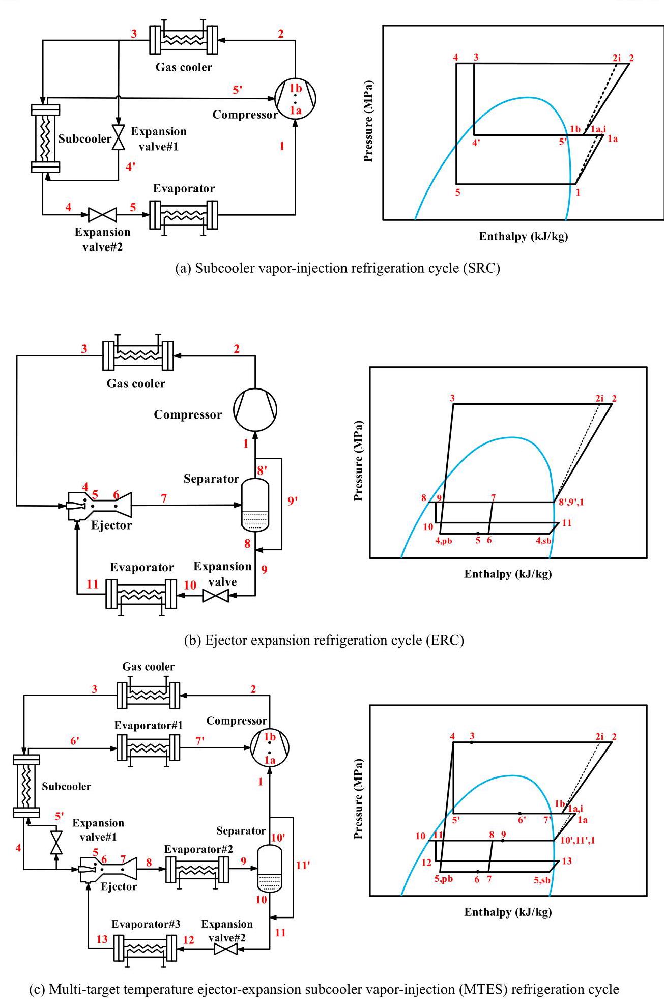
Fig. 1. Schematic configurations of the studied system.
2. System description
Schematic configurations of SRC, ERC and MTES refrigeration cycle are illustrated in Fig. 1. The SRC [24] cycle (Fig. 1(a)) consists of a compressor, a gas cooler, a subcooler, an evaporator and two expansion valves. Its main feature is to bypass a part of the refrigerant through expansion valve#1 for throttling expansion and then enter the sub-cooler, so that the temperature of the refrigerant entering expansion valve#2 is reduced, and the two-phase flow from expansion valve#1 is vaporized. The ERC [18] cycle (Fig. 1(b)) reduces the loss during throttling by adding ejector. The high-pressure supercritical ${\mathrm{{CO}}}_{2}$ fluid at the outlet of the gas cooler is used as the primary flow to drive the ejector. Then, the vapor leaving the ejector is divided into two phases in the separator. The gas-phase fluid enters the compressor, and the liquid-phase fluid enters the ejector as a secondary stream after passing through the evaporator. The proposed MTES cycle is shown in Fig. 1(c). The MTES cycle is a combination of SRC and ERC cycle. At the same time, the value of the $R$ of the SRC cycle and the $\omega$ of the ERC cycle are restricted, therefore, the multi-target temperature refrigeration is achieved by adding evaporator #1 after the subcooler and evaporator#2 after the ejector. Simultaneously, the addition of evaporator#1 and 2 removes the restriction of $R$ and $\omega$ .
3. Modeling for simulation and evaluation
3.1. Assumptions
This study will use the 1-D constant pressure model for the ejector calculation [29]. To simplify the theoretical model of the cycle, the following assumptions are made:
The flow through the ejector is regarded as a one-dimensional steady-state flow.
The pressure loss at the connection of each component and the speed of the fluid at the inlet and outlet of the ejector are ignored.
The primary flow and the secondary flow reach the same pressure at the inlet of the constant area and are constant pressure mixed in the mixing section.
The vapor flow in the gas-liquid separator is saturated vapor, and the liquid flow is saturated liquid.
The flow through the expansion valve is ideal isenthalpic expansion.
3.2. Two-phase flow ejector model
The use of an expansion energy recovery ejector has been given great concern owing to virtues of no moving elements, cost-effectiveness, high reliability, and comparable efficiency [15]. The first 1-D model describing the flow through the ejector was developed by Keenan et al. [30]. The authors proposed two different approaches to solve the flow. Mixing at constant pressure or constant area. Again, Keenan et al. [31] presented a more advanced method for both approaches mentioned before. In that case, the results reflected that constant pressure mixing was in a better agreement with experimental values. In this study, the 1-D constant pressure model for the ejector calculation was used, in which the state point in the formula is based on the MTES cycle as an example.
3.2.1. Ejector analysis
The mass flow rate ratio between the motive and suction fluid determines the entrainment ratio $\omega$ , which is used to evaluate the mass entrainment capacity of the ejector:
$$ \omega = \frac{{\dot{m}}_{s}}{{\dot{m}}_{P}} \tag{1} $$Table 1
Summary of theoretical and experimental values of two-phase ejector efficiency.
| Authors | Method | ${\eta }_{P}$ | ${\eta }_{s}$ | ${\eta }_{m}$ | ${\eta }_{d}$ |
| Elbel and Hrnjak (2004) [32] | Sim. | 0.9 | 0.9 | - | 0.9 |
| Li and Groll (2005) [18] | Sim. | 0.9 | 0.9 | - | 0.8 |
| Ksayer and Clodic (2006) [19] | Sim. | 0.85 | 0.85 | - | 0.75 |
| Deng et al. (2007) [33] | Sim. | 0.7 | 0.7 | - | 0.8 |
| Sarkar (2008) [34] | Sim. | 0.8 | 0.8 | - | 0.75 |
| Sun and Ma (2011) [17] | Sim. | 0.9 | 0.9 | - | 0.8 |
| Manjili and Yavari (2012) [35] | Sim. | 0.7 | 0.7 | 0.95 | 0.8 |
| Liu and Groll (2013) [13] | Exp. | 0.5-0.93 | 0.37-0.9 | 0.5-1 | - |
| Ahammed et al. (2014) [20] | Sim | 0.85 | 0.85 | - | 0.85 |
| Zheng et al. (2016) [36] | Sim. | 0.8 | 0.8 | 0.9 | 0.9 |
| Zheng et al. (2017) [37] | Exp. | 0.74-0.89 | ${0.86} - {0.96}$ | 0.73-0.9 | 0.75-0.95 |
| Taleghani and Sorin (2018) [38] | Sim. | 0.9 | 0.9 | 1 | 0.8 |
| Eskandari Manjili and Cheraghi (2019) [21] | Sim. | 0.9 | 0.9 | - | 0.8 |
| Zare and Rostamnejad Takleh (2020) [39] | Sim. | 0.9 | 0.9 | 0.88 | 0.85 |
| Peris Pérez et al. (2021) [40] | Sim. | 0.9 | 0.9 | 0.95 | 0.8 |
In addition, the various losses of the ejector are considered by the actual empirical efficiency, but a one-dimensional theoretical simulation is used in the present study. Therefore, constant coefficients will be used to characterize the theoretical performance of each section of the ejector. The theoretical and experimental values of the efficiency of the two-phase ejector used by previous scholars in the transcritical ${\mathrm{{CO}}}_{2}$ cycle are collected in Table 1. In this study, the smaller relative error between theoretical simulation and experimental data is considered. Motive and suction nozzles efficiencies around ${\eta }_{P} = {\eta }_{s} = {0.75}$ , mixing section efficiency around ${\eta }_{m} = {0.85}$ , and diffuser efficiency distribution around ${\eta }_{d} = {0.8}$ . The comparison of simulation and experimental results using these values is shown in section 3.6.
3.2.2. Primary and secondary nozzles
Primary flow expands with the given isentropic efficiency and gets accelerated to very high velocity. The conservation of energy and velocity at the exit of the primary nozzle are expressed by Eqs. (2) and (3).
$$ {h}_{P,5} = {h}_{4} - {\eta }_{P}\left( {{h}_{4} - h\left( {{P}_{5},{s}_{4}}\right) }\right) \tag{2} $$$$ {u}_{P,5} = \sqrt{2\left( {{h}_{4} - {h}_{P,5}}\right) } \tag{3} $$To create a vacuum at the ejector secondary flow nozzle, the pressure drop of the secondary nozzle is defined as:
$$ {\Delta P} = {P}_{e} - {P}_{5} \tag{4} $$The same method is used for the secondary nozzle as the primary nozzle. The conservation of energy and velocity at the exit of the secondary nozzle are expressed by Eqs. (5) and (6).
$$ {h}_{s,5} = {h}_{s,{13}} - {\eta }_{s}\left( {{h}_{s,{13}} - h\left( {{P}_{5},{s}_{s,{13}}}\right) }\right) \tag{5} $$$$ {u}_{s,5} = \sqrt{2\left( {{h}_{s,{13}} - {h}_{s,5}}\right) } \tag{6} $$3.2.3. Mixing section
The primary flow and secondary flow are mixed under constant pressure, the momentum and energy equations of the mixing process are:
$$ \left( {1 + \omega }\right) {u}_{6} = {u}_{P,5} + \omega {u}_{s,5} \tag{7} $$$$ \left( {1 + \omega }\right) \left( {{h}_{6, i} + \frac{{u}_{6, i}^{2}}{2}}\right) = \left( {1 + \omega }\right) \left( {{h}_{6} + \frac{{u}_{6}^{2}}{2}}\right) = \left\lbrack {\left( {{h}_{P,5} + \frac{{u}_{P,5}^{2}}{2}}\right) + \omega \left( {{h}_{s,5} + \frac{{u}_{s,5}^{2}}{2}}\right) }\right\rbrack $$(8)
The efficiency of the mixing section adopts a new mixing efficiency formula proposed by Ref. [41].
$$ {\eta }_{m} = \frac{\left( {1 + \omega }\right) {h}_{6, i} - {h}_{P,5} - \omega {h}_{s,5}}{\left( {1 + \omega }\right) {h}_{6} - {h}_{P,5} - \omega {h}_{s,5}} = \frac{{u}_{P,5}^{2} + \omega {u}_{s,5}^{2} - \left( {1 + \omega }\right) {u}_{6, i}^{2}}{{u}_{P,5}^{2} + \omega {u}_{s,5}^{2} - \left( {1 + \omega }\right) {u}_{6}^{2}} \tag{9} $$3.2.4. Shock section
Considering that ${\mathrm{{CO}}}_{2}$ in transcritical conditions is entering the primary nozzle, it is likely that the fluid will reach the speed of sound during the mixing process, which will result in a normal shock in the constant area section [42]. presented a simple model for predicting the sonic velocity in two-phase systems. The model has shown to be remarkably successful in predicting the sonic velocity in most of the flow regimes of two-phase gas-liquid flows over the entire range of void and mass fraction. The void fraction and the sound velocity of the two-phase flow are defined as Eqs. (10) and (11).
$$ \alpha = \frac{X{\rho }_{L}}{X{\rho }_{L} + \left( {1 + X}\right) {\rho }_{G}} \tag{10} $$$$ C = \frac{1}{\left( {1 - \alpha }\right) \sqrt{\frac{1 - \alpha }{{C}_{L}^{2}} + \frac{\alpha {\rho }_{L}}{{\rho }_{G}{C}_{G}^{2}}} + \alpha \sqrt{\frac{\alpha }{{C}_{G}^{2}} + \frac{\left( {1 - \alpha }\right) {\rho }_{G}}{{\rho }_{L}{C}_{L}^{2}}}} \tag{11} $$If the speed of ${\mathrm{{CO}}}_{2}$ after the mixing process is greater than the speed of sound, Eqs. 12-14 is used to express the impact of the shock wave. Otherwise, all the characteristics of the refrigerants remain unchanged. Conservation of mass, momentum, and energy:
$$ {\rho }_{6}{u}_{6} = {\rho }_{7}{u}_{7} \tag{12} $$$$ {P}_{6} + {\rho }_{6}{u}_{6}^{2} = {P}_{7} + {\rho }_{7}{u}_{7}^{2} \tag{13} $$$$ {h}_{6} + \frac{{u}_{6}^{2}}{2} = {h}_{7} + \frac{{u}_{7}^{2}}{2} \tag{14} $$The relationship of the density change during the shock wave is expressed:
$$ {\rho }_{7} = {\rho }_{6}\frac{\left( {1 + k}\right) {M}_{6}^{2}}{\left( {k - 1}\right) {M}_{6}^{2} + 2} \tag{15} $$In which $k$ for two-phase:
$$ k = {X}_{6}\frac{{C}_{P}\left( {{P}_{6}, X = 1}\right) }{{C}_{V}\left( {{P}_{6}, X = 1}\right) } + \left( {1 - {X}_{6}}\right) \frac{{C}_{P}\left( {{P}_{6}, X = 0}\right) }{{C}_{V}\left( {{P}_{6}, X = 0}\right) } \tag{16} $$3.2.5. Diffuser section
In the diffusion section, the fluid loses kinetic energy, causing the fluid pressure to increase. The formula is:
$$ {h}_{8} = {h}_{7} + \frac{{u}_{7}^{2}}{2} = \frac{{h}_{4} + \omega {h}_{13}}{\left( 1 + \omega \right) } \tag{17} $$$$ {h}_{8, i} = {h}_{7} + {\eta }_{d}\left( {{h}_{8} - {h}_{7}}\right) \tag{18} $$Table 2
Thermodynamic equations of the studied refrigeration systems.
| Refrigeration system | Component | Thermodynamic balance equation |
| SRC | Compressor | ${s}_{{1a}, i} = {s}_{1},{s}_{2, i} = {s}_{1b},{\eta }_{c, L} = \frac{{h}_{{1a}, i} - {h}_{1}}{{h}_{1a} - {h}_{1}},$ |
| ${\eta }_{c, H} = \frac{{h}_{2, i} - {h}_{1b}}{{h}_{2} - {h}_{1b}}$ $\dot{W} = \dot{m}\left( {1 - R}\right) \left( {{h}_{1a} - {h}_{1}}\right) + \dot{m}\left( {{h}_{2} - {h}_{1b}}\right)$ | ||
| Gas cooler | ${\dot{Q}}_{gc} = \dot{m}\left( {{h}_{2} - {h}_{3}}\right)$ | |
| Subcooler | $\dot{m}\left( {R - 1}\right) \left( {{h}_{3} - {h}_{4}}\right) = \dot{m}R\left( {{h}_{{5}^{\prime }} - {h}_{{4}^{\prime }}}\right)$ | |
| Expansion valve#1 | ${h}_{3} = {h}_{{4}^{\prime }}$ | |
| Expansion valve#2 | ${h}_{4} = {h}_{5}$ | |
| Evaporator | ${\dot{Q}}_{e} = \dot{m}\left( {1 - R}\right) \left( {{h}_{1} - {h}_{5}}\right)$ | |
| ERC | Compressor | ${s}_{2, i} = {s}_{1},{\eta }_{c} = \frac{{h}_{2, i} - {h}_{1}}{{h}_{2} - {h}_{1}},\dot{W} = \dot{m}\left( {{h}_{2} - {h}_{1}}\right)$ |
| Gas cooler | ${\dot{Q}}_{gc} = \dot{m}\left( {{h}_{2} - {h}_{3}}\right)$ | |
| Ejector | $\left( {1 + \omega }\right) {h}_{7} = {h}_{3} + \omega {h}_{11}$ | |
| Expansion valve | ${h}_{9} = {h}_{10}$ | |
| Evaporator | ${\dot{Q}}_{e} = \dot{m}\omega \left( {1 - R}\right) \left( {{h}_{11} - {h}_{10}}\right)$ | |
| MTES | Compressor | ${s}_{{1a}, i} = {s}_{1},{s}_{2, i} = {s}_{1b},{\eta }_{c, L} = \frac{{h}_{{1a}, i} - {h}_{1}}{{h}_{1a} - {h}_{1}},$ |
| ${\eta }_{c, H} = \frac{{h}_{2, i} - {h}_{1b}}{{h}_{2} - {h}_{1b}}$ | ||
| $\dot{W} = \dot{m}\left( {1 - R}\right) \left( {{h}_{1a} - {h}_{1}}\right) + \dot{m}\left( {{h}_{2} - {h}_{1b}}\right)$ | ||
| Gas cooler | ${\dot{Q}}_{gc} = \dot{m}\left( {{h}_{2} - {h}_{3}}\right)$ | |
| Subcooler | $\dot{m}\left( {{h}_{3} - {h}_{4}}\right) = \dot{m}R\left( {{h}_{{6}^{\prime }} - {h}_{{5}^{\prime }}}\right)$ | |
| Ejector | $\left( {1 + \omega }\right) {h}_{8} = {h}_{4} + \omega {h}_{13}$ | |
| Expansion valve#1 | ${h}_{4} = {h}_{{5}^{\prime }}$ | |
| Expansion valve#2 | ${h}_{11} = {h}_{12}$ | |
| Evaporator#2 | ${\dot{Q}}_{e1} = \dot{m}R\left( {{h}_{{7}^{\prime }} - {h}_{{6}^{\prime }}}\right)$ | |
| Evaporator#3 | ${\dot{Q}}_{e2} = \dot{m}\left( {1 - R}\right) \left( {1 + \omega }\right) \left( {{h}_{9} - {h}_{8}}\right)$ | |
| Evaporator#3 | ${\dot{Q}}_{e3} = \dot{m}\omega \left( {1 - R}\right) \left( {{h}_{13} - {h}_{12}}\right)$ |
3.3. Energetic analysis
The general energy balance equation can be defined as:
$$ {\dot{Q}}_{i} - {\dot{W}}_{o} + \sum {\dot{m}}_{i}{h}_{i} - \sum {\dot{m}}_{o}{h}_{o} = 0 \tag{19} $$where ${\dot{Q}}_{i}$ means the net heat input rate of each component while ${\dot{W}}_{o}$ means the net work output rate of each component, $\dot{m}$ is the mass flow rate of the working fluid. By using Eq. (19), the thermodynamic equations of each component of the aforementioned systems are obtained as shown in Table 2.
The mass flow rate ratio between the bypass and main cycle fluid determines the bypass mass ratio $R$ .
$$ R = \frac{{m}_{5}}{{m}_{4}} \tag{20} $$The intermediate pressure is obtained from the classical estimated value, given by the geometric mean of discharge pressure and evaporating pressure [43].
$$ {P}_{\text{ int }} = \sqrt{{P}_{\text{ dis }}{P}_{e3}} \tag{21} $$The compression and expansion processes follow the modeling assumptions. In addition, to simplify the calculation, the mass flow through the compressor is the unit mass " ${\dot{m}}^{\prime \prime }\left( {\dot{m} = 1\mathrm{\;{kg}}/\mathrm{s}}\right)$ . The isentropic efficiency expressions of compressor is expressed in the following equations [44]:
$$ {\eta }_{c} = {0.8981} - {0.09238CR} + {0.00476C}{R}^{2} \tag{22} $$The evaluation parameter in terms of energetic performance is then given as refrigerating cycle COP.
$$ {COP} = \frac{\sum \dot{Q}}{\sum \dot{W}} \tag{23} $$Table 3
The exergy destruction calculation equation for each component.
| Refrigeration system | Component | Exergy destruction |
| SRC | Compressor | $\dot{E}{x}_{D, c} = \dot{m}{T}_{0}\left\lbrack {\left( {1 - R}\right) \left( {{s}_{1a} - {s}_{1}}\right) + \left( {{s}_{2} - {s}_{1b}}\right) }\right\rbrack$ |
| Gas cooler | $\dot{E}{x}_{D,{gc}} = \dot{m}\left\lbrack {\left( {{h}_{2} - {h}_{3}}\right) - {T}_{0}\left( {{s}_{2} - {s}_{3}}\right) }\right\rbrack$ | |
| Subcooler | $\dot{E}{x}_{D, s} = \dot{m}\left( {1 - R}\right) \left\lbrack {\left( {{h}_{3} - {h}_{4}}\right) - {T}_{0}\left( {{s}_{3} - {s}_{4}}\right) }\right\rbrack + \; \dot{m}R\left\lbrack {\left( {{h}_{{4}^{\prime }} - {h}_{{5}^{\prime }}}\right) - {T}_{0}\left( {{s}_{{4}^{\prime }} - {s}_{{5}^{\prime }}}\right) }\right\rbrack$ | |
| Expansion valve#1 | $\dot{E}{x}_{D,{ev1}} = \dot{m}R{T}_{0}\left\lbrack \left( {{s}_{{4}^{\prime }} - {s}_{3}}\right) \right\rbrack$ | |
| Expansion valve#2 | $\dot{E}{x}_{D,{ev2}} = \dot{m}\left( {1 - R}\right) {T}_{0}\left\lbrack \left( {{s}_{5} - {s}_{4}}\right) \right\rbrack$ | |
| Evaporator | $\dot{E}{x}_{D, e} = \dot{m}{T}_{0}\left\lbrack {\frac{1}{{T}_{e} + {T}_{sh}}\left( {{h}_{5} - {h}_{1}}\right) - \left( {{s}_{5} - {s}_{1}}\right) }\right\rbrack$ | |
| ERC | Compressor | $\dot{E}{x}_{D, c} = \dot{m}{T}_{0}\left( {{s}_{2} - {s}_{1}}\right)$ |
| Gas cooler | $\dot{E}{x}_{D,{gc}} = \dot{m}\left\lbrack {\left( {{h}_{2} - {h}_{3}}\right) - {T}_{0}\left( {{s}_{2} - {s}_{3}}\right) }\right\rbrack$ | |
| Ejector | $\dot{E}{x}_{D,{ej}} = \dot{m}{T}_{0}\left\lbrack {\left( {1 + \omega }\right) {s}_{7} - {s}_{3} - \omega {s}_{11}}\right\rbrack$ | |
| Expansion valve | $\dot{E}{x}_{D,{ev}} = \dot{m}{T}_{0}\omega \left\lbrack \left( {{s}_{10} - {s}_{9}}\right) \right\rbrack$ | |
| Evaporator | $\dot{E}{x}_{D, e} = \dot{m}\omega {T}_{0}\left\lbrack {\frac{1}{{T}_{e} + {T}_{sh}}\left( {{h}_{10} - {h}_{11}}\right) -({s}_{10} - }\right. \; \left. \left. {s}_{11}\right) \right\rbrack$ | |
| MTES | Compressor | $\dot{E}{x}_{D, c} = \dot{m}{T}_{0}\left( {1 - R}\right) \left( {{s}_{1a} - {s}_{1}}\right) + \dot{m}{T}_{0}\left( {{s}_{2} - }\right. \; {s}_{1b})$ |
| Gas cooler | $\dot{E}{x}_{D,{gc}} = \dot{m}\left\lbrack {\left( {{h}_{2} - {h}_{3}}\right) - {T}_{0}\left( {{s}_{2} - {s}_{3}}\right) }\right\rbrack$ | |
| Subcooler | $\dot{E}{x}_{D, s} = \dot{m}\left\lbrack {\left( {{h}_{3} - {h}_{4}}\right) - {T}_{0}\left( {{s}_{3} - {s}_{4}}\right) }\right\rbrack + \; \dot{m}R\left\lbrack {\left( {{h}_{{5}^{\prime }} - {h}_{{6}^{\prime }}}\right) - {T}_{0}\left( {{s}_{{5}^{\prime }} - {s}_{{6}^{\prime }}}\right) }\right\rbrack$ | |
| Ejector | $\dot{E}{x}_{D,{ej}} = \dot{m}{T}_{0}\left( {1 - R}\right) \left\lbrack {\left( {1 + \omega }\right) {s}_{8} - {s}_{4} - \omega {s}_{13}}\right\rbrack$ | |
| Expansion valve#1 | $\dot{E}{x}_{D,{ev1}} = \dot{m}R{T}_{0}\left\lbrack \left( {{s}_{{5}^{\prime }} - {s}_{4}}\right) \right\rbrack$ | |
| Expansion valve#2 | $\dot{E}{x}_{D,{ev2}} = \dot{m}\omega {T}_{0}\left( {1 - R}\right) \left\lbrack \left( {{s}_{12} - {s}_{11}}\right) \right\rbrack$ | |
| Evaporator#2 | $\dot{E}{x}_{D,{e1}} = \dot{m}R{T}_{0}\left\lbrack {\frac{1}{{T}_{e1}}\left( {{h}_{{6}^{\prime }} - {h}_{{7}^{\prime }}}\right) - \left( {{s}_{{6}^{\prime }} - {s}_{{7}^{\prime }}}\right) }\right\rbrack$ | |
| Evaporator#3 | $\dot{E}{x}_{D,{e2}} = \dot{m}\left( {1 + \omega }\right) \left( {1 - R}\right) {T}_{0}\left\lbrack {\frac{1}{{T}_{e2}}\left( {{h}_{8} - {h}_{9}}\right) - }\right.$ | |
| $\left. \left( {{s}_{8} - {s}_{9}}\right) \right\rbrack$ | ||
| Evaporator#3 | $\dot{E}{x}_{D,{e3}} = \dot{m}\omega \left( {1 - R}\right) {T}_{0}\left\lbrack {\frac{1}{{T}_{e3} + {T}_{sh}}\left( {{h}_{12} - }\right. }\right. \; \left. {\left. {h}_{13}\right) - \left( {{s}_{12} - {s}_{13}}\right) }\right\rbrack$ |
3.4. Exergetic analysis
Evaluation of a system also includes the various exergy destructions of various components. Thus, exergetic analysis is applied in this study. The specific exergy of the refrigerant at every state point can be defined as [45]:
$$ {ex} = \left( {h - {h}_{0}}\right) - {T}_{0}\left( {s - {s}_{0}}\right) \tag{24} $$where the subscript 0 represents the reference state which is selected as 300.15K under the ambient atmosphere pressure 101.325 kPa. Based on the second law of thermodynamics, the exergy destruction in each component can be calculated by following equation:
$$ \dot{E}{x}_{D} = \dot{E}{x}_{Q} - \dot{E}{x}_{W} + \sum {\dot{m}}_{i}e{x}_{i} - \sum {\dot{m}}_{o}e{x}_{o} \tag{25} $$Based on the above two equations, the exergy destruction in each component of the systems can be obtained and is listed in Table 3. In addition, the cycle total exergy destruction can be obtained as:
$$ \dot{E}{x}_{D, t} = \mathop{\sum }\limits_{k}\dot{E}{x}_{D, k} \tag{26} $$The exergy efficiency is defined as the ratio of the effective exergy output to the effective exergy input, where the effective exergy output can be obtained by subtracting the total exergy loss from the effective exergy input. The system exergy efficiency is expressed as follows [46]:
$$ {\eta }_{Ex} = 1 - \frac{\mathop{\sum }\limits_{k}\dot{E}{x}_{D, k}}{\mathop{\sum }\limits_{k}{\dot{W}}_{{in}, k}} \tag{27} $$3.5. Model procedure
The flow chart of the MTES cycle simulation program is shown in Fig. 2. In this study, the performance of the MTES cycle is affected through four design variables. The variables include the gas cooler outlet temperature $\left( {T}_{gc}\right)$ , evaporating temperature of evaporator#3 $\left( {T}_{e3}\right)$ , the entrainment rate of ejector $\left( \omega \right)$ and the bypass mass ratio $\left( R\right)$ . Based on the set working conditions, the range of each variable is as follows:
$$ {35}^{ \circ }C \leq {T}_{gc} \leq {45}^{ \circ }C \tag{28} $$$$
- {30}^{ \circ }C \leq {T}_{e3} \leq {0}^{ \circ }C \tag{29} $$
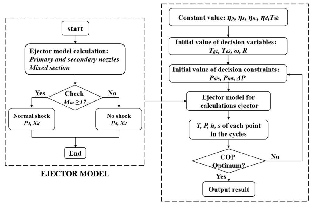
Fig. 2. The flow chart of the program.
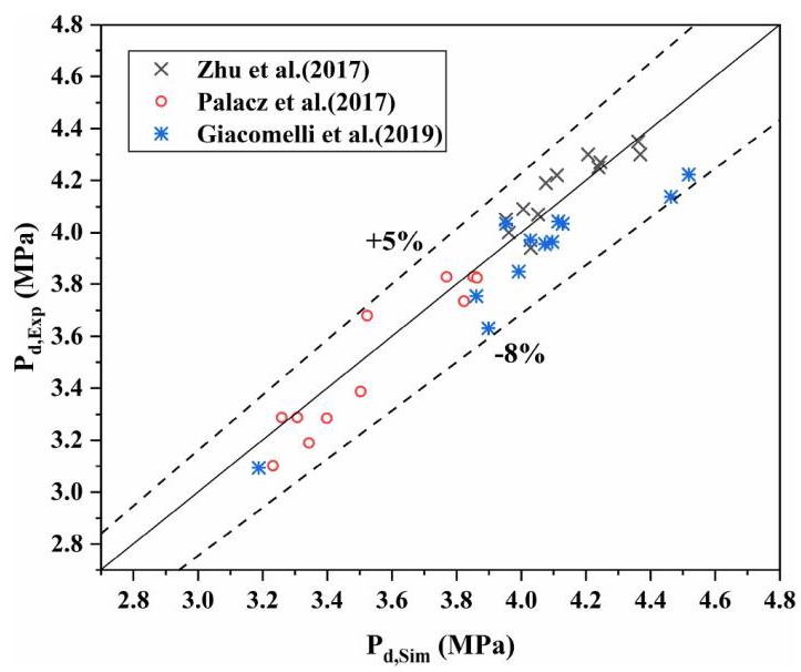
Fig. 3. Comparison of simulated and experimental values of ejector model.
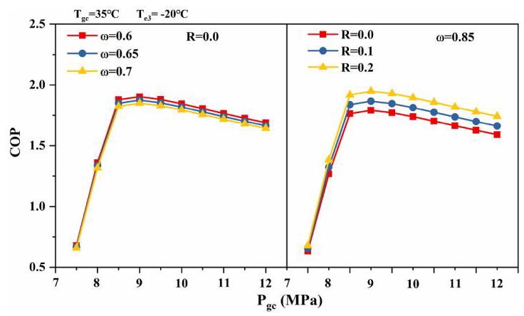
Fig. 4. The effect of the $\omega$ and $\mathrm{R}$ on the optimal discharge pressure.
In this study, the compressor discharge pressure $\left( {P}_{dis}\right)$ , the intermediate pressure $\left( {P}_{\text{ int }}\right)$ and the pressure drop of the secondary nozzle $\left( {\Delta P}\right)$ are taken as the constraints. The optimal value of COP is calculated in MATLAB R2017b based on the Genetic Algorithm Multi-objective simulation model. The thermodynamic data are used REFPROP 9.1 for thermodynamic state and characteristic calculation. In addition to the basic algorithm, it also includes iteration conditions and variable values, the required thermodynamic parameters are calculated.
3.6. Model validation
To validate the accuracy of the proposed model of two-phase flow ejector and efficiency assumptions, operating data reported in the literature using ${\mathrm{{CO}}}_{2}$ are considered [47-49]. Specifically,36 sets of experimental data are selected, and the results obtained by the model calculation are compared with the experimental data in the literature, which are collected in Table 5. The pressure and temperature of the ejector’s primary and secondary flow are given in the experimental data, and the ejector outlet pressure and entrainment rate are also provided. The ejector outlet pressure is calculated by simulation and compared with the experimental values. The comparison result is shown along with the error bandwidth of the prediction. It can be seen from Fig. 3 that the error is between -8% and +5%. However, considering the constant efficiency assumption is to simplify the model, therefore, the error range can be acceptable, and the mathematical model is considered accurate enough for this investigation.
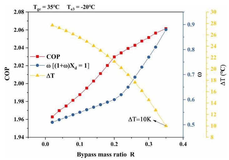
Fig. 5. Variation of $\omega ,\mathrm{{COP}},{\Delta T}$ with $R$ (MTES).
4. Results and discussion
4.1. MTES cycle behavior
4.1.1. Effect of discharge pressure
The optimal discharge pressure is one of the indispensable parameters when discussing the transcritical ${\mathrm{{CO}}}_{2}$ cycle. Fig. 4 shows the effect of $\omega$ and $R$ on the optimal exhaust pressure for the MTES cycle. The variation trend of COP with the optimal discharge pressure is also in line with the characteristics of typical transcritical ${\mathrm{{CO}}}_{2}$ systems: the COP increases with the increase of ${\mathrm{P}}_{\mathrm{{gc}}}$ , and COP gradually decreases after the optimal pressure is reached. It can be observed from Fig. 4 that the $\omega$ and $R$ have little effect on the optimal discharge pressure, the optimum discharge pressure is always around ${9.0}\mathrm{{MPa}}$ as the change of $\omega$ and $R$ values.
4.1.2. Effect of evaporating temperature, cooling capacity and COP
The MTES cycle includes an ejector and vapor-injection. there are two restrictive conditions in the MTES cycle in order to ensure a constant vapor mass flow at the compressor inlet when the evaporator 1 and 2 are in a non-operating state.
The vapor quality at the ejector outlet must meet a condition: $(1 + \; \omega ){X}_{d} \geq 1$ , in other words, the minimum entrainment rate $\left( {\omega }_{\min }\right)$ is limited by this condition.
The value of $R$ is related to the heat exchange temperature difference $\left( {{\Delta T} = {T}_{4} - {T}_{{5}^{\prime }}}\right)$ of the subcooler, that is to ensure ${\Delta T} \geq {10}^{ \circ }\mathrm{C}$ .
Based on the above two restrictions, the variation of $\omega$ , COP and ${\Delta T}$ with $R$ is shown in Fig. 5. The operating conditions are given as follows: the gas cooler outlet temperature ${T}_{gc} = {35}^{ \circ }\mathrm{C}$ , evaporating temperature of evaporator#3 ${T}_{e3} = - {20}^{ \circ }\mathrm{C}$ and the evaporator superheating degree ${T}_{sh} = {5}^{ \circ }\mathrm{C}$ . It can be seen that the COP of the MTES cycle increases with the increase of $R$ , which reflects that vapor-injection is positive for cycle performance, because vapor-injection reduces compressor power consumption. The value of $\omega$ increases as the $R$ is rised, the reason is that the fluid temperature at the inlet of the primary nozzle of the ejector is reduced as the value of $R$ increases, the value of $\omega$ must be increased to ensure sufficient vapor quality at the compressor inlet. In addition, the value of $R$ is restricted by ${\Delta T}$ , it can be seen from Fig. 5 that $R$ reaches the maximum value of 0.35 when ${\Delta T} = {10}^{ \circ }\mathrm{C}$ under this operating condition.
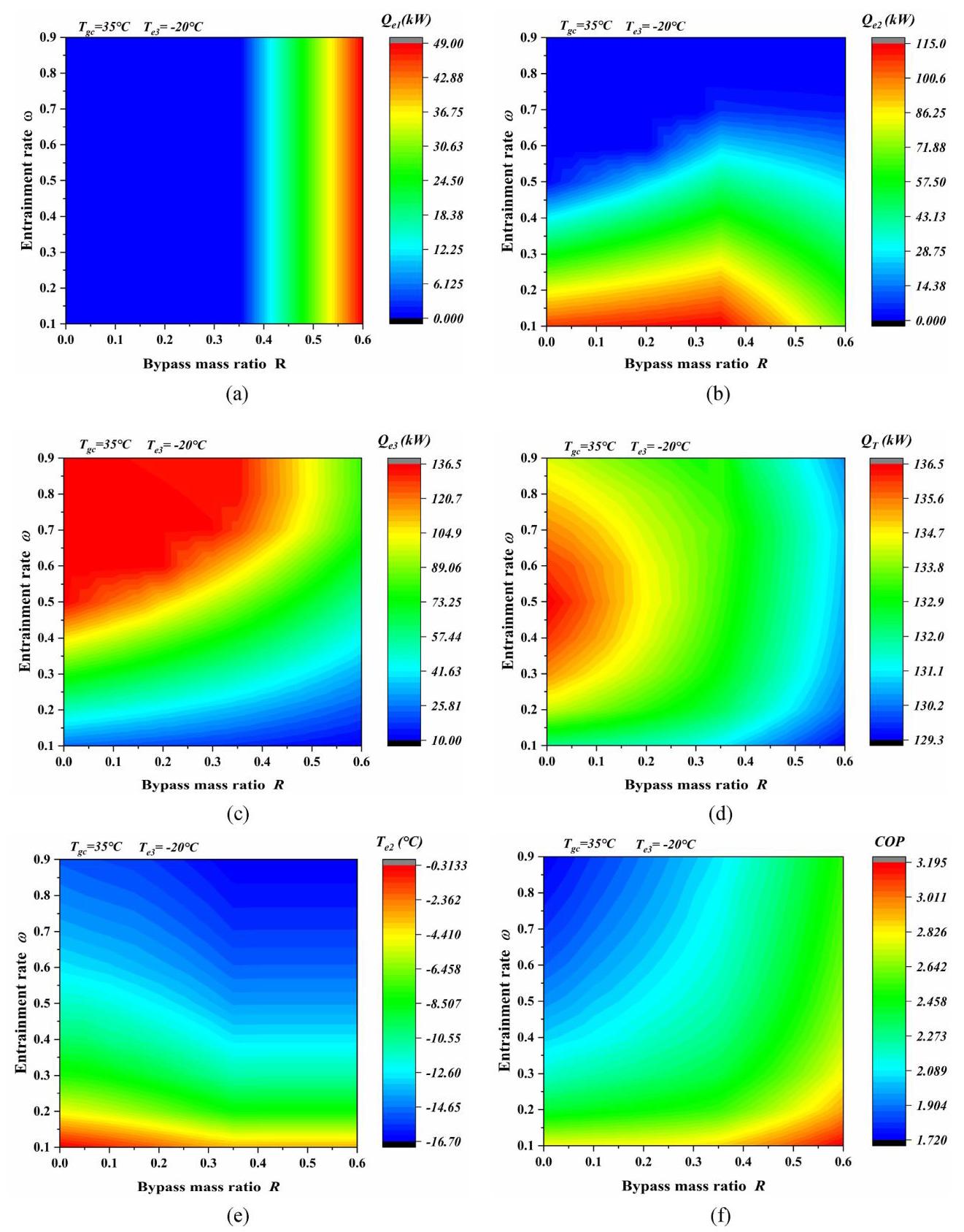
Fig. 6. The effect of the $\omega$ and $R$ on other parameters. (a) effect on ${Q}_{e1}$ ; (b) effect on ${Q}_{e2}$ ; (c) effect on ${Q}_{e3}$ ; (d) effect on ${Q}_{r2}$ ; (e) effect on ${T}_{e2}$ ; (f) effect on COP.
Based on the two restrictions of $\omega$ and $R$ discussed above, evaporator#1 and evaporator#2 were added to break the two restrictions and achieve multi-target temperature refrigeration. The following will discuss the characteristics of the MTES cycle in multi-target temperature refrigeration, where three parameters including the evaporating temperature of each evaporator, the cooling capacity of each evaporator and the COP are studied.
Fig. 6(a) depicts the variation of cooling capacity of evaporator#1 on the $R$ and the $\omega$ . It can be seen that the value of ${\dot{Q}}_{e1}$ increases as the $R$ is rised when $R \geq {0.35}$ under this operating condition, and the value of ${\dot{Q}}_{e1}$ is irrelevant to $\omega$ . The reason is that the refrigerant in the bypass cannot completely become saturated vapor when $R \geq {0.35}$ , therefore, the cooling capacity ${\dot{Q}}_{e1}$ of the evaporator#1 will gradually increase to ensure that the intermediate vapor injected into the compressor is in the vapor state.
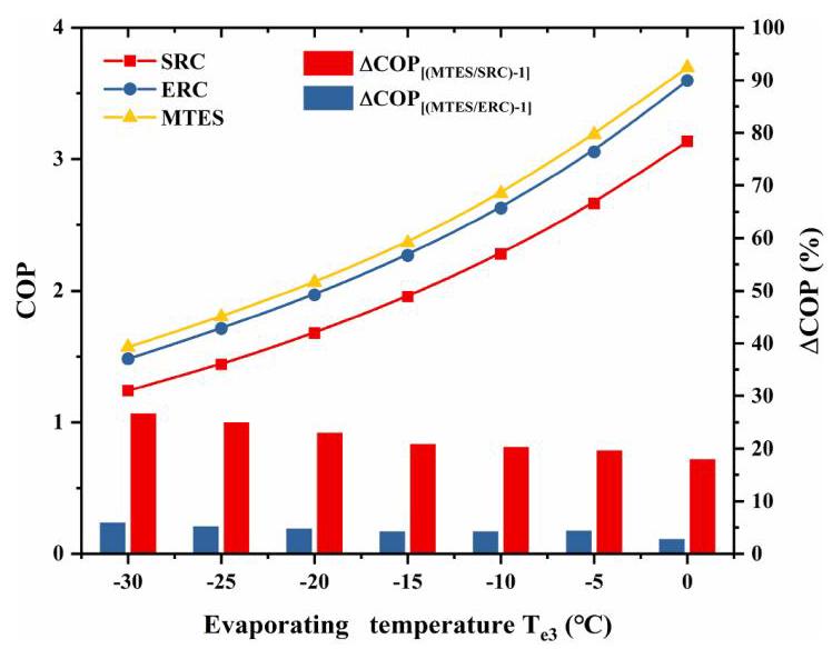
Fig. 7. Variation of COP with evaporating temperature for SRC, ERC and MTES cycles $\left( {{\mathrm{T}}_{\mathrm{{gc}}} = {35}^{ \circ }\mathrm{C}}\right)$ .
Fig. 6(b) illustrates the variation of cooling capacity of evaporator#2 on the $R$ and the $\omega$ . The following points can be seen:
a) The value of ${\omega }_{\min }$ increases as the $R$ is rised when $R < {0.35}$ ; the value of ${\omega }_{\min }$ remains constant as the $R$ is rised when $R \geq {0.35}$ . Specifically, the fluid temperature at the inlet of the primary nozzle of the ejector is remained constant when $R \geq {0.35}$ , therefore, the value of ${\omega }_{\min }$ does not continue to increase.
b) The value of ${\dot{Q}}_{e2}$ increases as the $\omega$ is reduced when the value of $R$ is constant; the value of ${\dot{Q}}_{e2}$ increases as the $R$ is rised when the value of $\omega$ is constant and $R < {0.35}$ . The reason is that with the decrease of $\omega$ and the increase of $R$ , the vapor quality at the ejector outlet continues to decrease, the refrigeration capacity of evaporator#2 is increased.
c) The value of ${\dot{Q}}_{e2}$ decreases as the $R$ is rised when the value of $\omega$ is constant and $R \geq {0.35}$ . Specifically, the inlet state of the primary nozzle and the secondary nozzle of the ejector does not change. At this time, when $R$ gradually increases, the mass flow rate of the ejector outlet decreases, which leads to a decrease in ${\dot{Q}}_{e2}$ .
Fig. 6(c) represents the variation of cooling capacity of evaporator#3 on the $R$ and the $\omega$ . It can be seen that the value of ${\dot{Q}}_{e3}$ decreases as the $\omega$ is reduced when the value of $R$ is constant, the mass flow through the evaporator#3 is reduced because $\omega$ is reduced, which leads to a reduction in ${\dot{Q}}_{e3}$ .
Fig. 6(d) shows the variation of total cooling capacity of evaporator on the $R$ and the $\omega$ . It can be seen that the $R$ and $\omega$ parameters have little effect on the ${\dot{Q}}_{T}$ .
For the evaporating temperature of the evaporator#1, evaporator#2 and evaporator#3:
a) The evaporating temperature of the evaporator#1 is determined by the pressure on the high and low pressure sides. The problem can be written as follows: ${T}_{e1} = f\left( {{P}_{\text{ int }},{X}_{{7}^{\prime }} = 1}\right)$ . The high and low pressures remain unchanged under the conditions discussed in this section, so ${T}_{e1}$ remains constant.
b) Fig. 6(e) shows the variation of the evaporating temperature of the evaporator#2 on the $R$ and the $\omega$ . It can be seen that the value of ${T}_{e2}$ increases as the $\omega$ is reduced when the value of $R$ is constant. The value of ${T}_{e2}$ decreases as the $R$ is rised when $R < {0.35}$ ; the value of ${T}_{e2}$ remains constant as the $R$ is rised when $R \geq {0.35}$ .
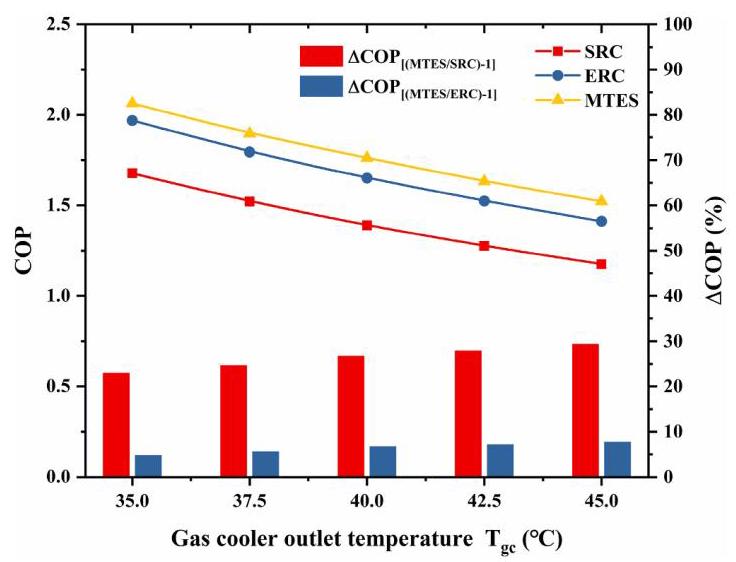
Fig. 8. Variation of COP with gas cooler outlet temperature for SRC, ERC and MTES cycles $\left( {{\mathrm{T}}_{e3} = - {20}^{ \circ }\mathrm{C}}\right)$ .
c) The evaporating temperature of the evaporator#3 is set to a constant value $\left( {{T}_{e3} = - {20}^{ \circ }\mathrm{C}}\right)$ .
Finally, Fig. 6(f) shows the variation of COP of cycle on the $R$ and the $\omega$ . It can be seen that the value of COP increases as the $\omega$ is reduced, and the value of COP increases as the $R$ is rised. As analyzed above, a part of the refrigerant becomes gaseous at the evaporating temperature ${T}_{e1}$ and ${T}_{e2}$ when the evaporator#1 and the evaporator#2 are working, which causes the compressor intake pressure to rise, and then the COP increases.
4.2. Comparison of SRC, ERC and MTES cycles
To evaluate the thermodynamic performance of the MTES cycle, under the same operating conditions (evaporator#1 and evaporator#2 of the MTES cycle are not operating), the advantages of the MTES cycle are described by comparing the COP and exergy efficiency of SRC, ERC and MTES cycles.
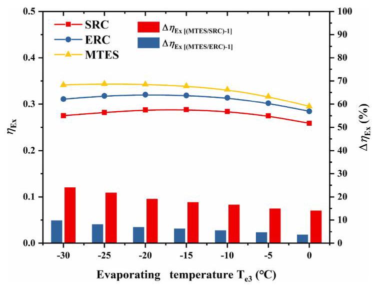
Fig. 9. Variation of ${\eta }_{Ex}$ with evaporating temperature for SRC, ERC and MTES cycles $\left( {{\mathrm{T}}_{\mathrm{{gc}}} = {35}^{ \circ }\mathrm{C}}\right)$ .
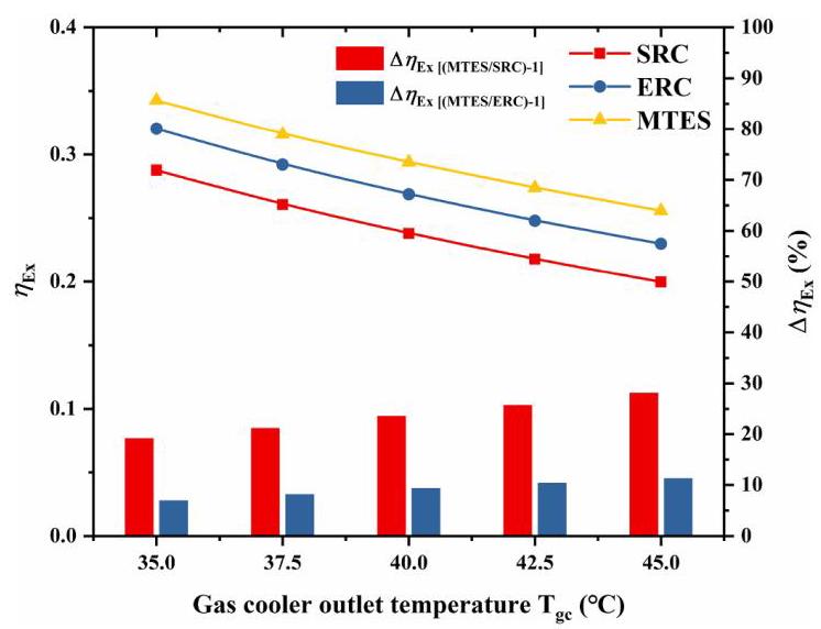
Fig. 10. Variation of ${\eta }_{Ex}$ with gas cooler temperature for SRC, ERC and MTES cycles $\left( {{T}_{e3} = - {20}^{ \circ }\mathrm{C}}\right)$ .
4.2.1. Parametric analysis on the COP of the SRC, ERC and MTES cycles
Fig. 7 shows the COP comparison between SRC, ERC and MTES cycles within the selected evaporating temperature range. As expected, the value of COP decreases as the evaporating temperature is reduced. Compared with SRC and ERC systems, the MTES cycle shows higher COP when applied to the selected temperature range. Specifically, the COP of the MTES cycle in the study temperature range is 17.9-26.7% higher than that of SRC cycle, and 2.8-6% higher than that of ERC cycle, respectively. In addition, the value of ΔCOP increases as the evaporating temperature is reduced, it shows that the MTES cycle performs better under low temperature conditions.
Fig. 8 shows the COP comparison of SRC, ERC and MTES cycles with the change of gas cooler outlet temperature. As expected, the value of COP decreases as the gas cooler outlet temperature is rised. As can be observed, the COP of the MTES cycle in the study temperature range is 23-29.4% higher than that of SRC cycle, and 4.8-7.8% higher than that of ERC cycle, respectively. The value of ΔCOP increases as the gas cooler outlet temperature is rised, which means that the MTES cycle has a more competitive advantage under high ambient temperature conditions.
4.2.2. Parametric analysis on the exergy efficiency of the SRC, ERC and MTES cycles
Fig. 9 illustrates a comparison between the exergy efficiency of the cycles at different evaporating temperatures. The value of ${\eta }_{Ex}$ changes little with the evaporation temperature, the main reason is that the total system exergy loss and the compressor power decrease, and the rate of decrease of the two is similar. In addition, it can be seen that MTES cycle has higher exergy efficiency than SRC and ERC cycles. Specifically, the ${\eta }_{Ex}$ of the MTES cycle in the study temperature range is ${14} - {24}\%$ higher than that of SRC cycle, and 3.7-9.8% higher than that of ERC cycle, respectively. The variation trend of $\Delta {\eta }_{Ex}$ with evaporating temperature is similar to $\Delta \mathrm{{COP}}$ in Fig. 7.
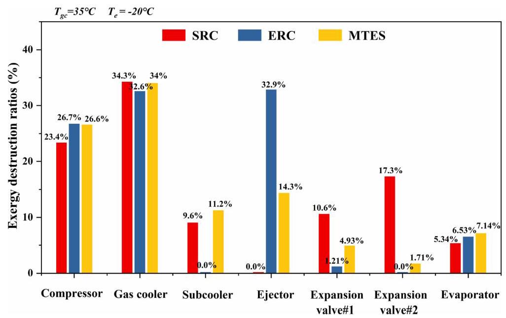
Fig. 11. Exergy destruction ratios of different component varieties for SRC, ERC and MTES cycles.
Table 4
Exergy destruction in cycles $\left( {{\mathrm{T}}_{\mathrm{{gc}}} = {35}^{ \circ }\mathrm{C},{\mathrm{T}}_{\mathrm{e}} = - {20}^{ \circ }\mathrm{C}}\right)$ .
| Component | SRC Exergy destruction rate (kJ/ kg) | Percentage (%) | ERC Exergy destruction rate (kJ/ kg) | Percentage (%) | MTES Exergy destruction rate (kJ/ kg) | Percentage (%) |
| Compressor | 10.78 | 23.39 | 12.13 | 26.74 | 11.03 | 26.59 |
| Gas cooler | 15.80 | 34.27 | 14.78 | 32.59 | 14.11 | 34.03 |
| Subcooler | 4.17 | 9.06 | - | - | 4.67 | 11.25 |
| Ejector | - | - | 14.92 | 32.89 | 5.95 | 14.35 |
| Expansion valve#1 | 4.89 | 10.61 | 0.55 | 1.21 | 2.05 | 4.93 |
| Expansion valve#2 | 7.98 | 17.32 | - | - | 0.71 | 1.71 |
| Evaporator | 2.46 | 5.34 | 2.98 | 6.50 | 2.96 | 7.14 |
| Total | 46.09 | 45.37 | 41.47 |
Table 5
Experimental data and results of the model validation.
| Case | Primary nozzle | Secondary nozzle | Outlet results | Ref. | |||||
| ${P}_{P}\left( \mathrm{{MPa}}\right)$ | ${T}_{P}\left( {{}^{ \circ }\mathrm{C}}\right)$ | ${P}_{s}\left( \mathrm{{MPa}}\right)$ | ${T}_{s}\left( {{}^{ \circ }\mathrm{C}}\right)$ | ${m}_{P}\left( {\mathrm{\;{kg}}/\mathrm{h}}\right)$ | $\omega$ | ${P}_{d,{Exp}}\left( \mathrm{{MPa}}\right)$ | ${P}_{d,{Sim}}\left( \mathrm{{MPa}}\right)$ | ||
| 1 | 8.15 | 35.3 | 3.63 | 24.0 | 61.35 | 0.38 | 4.30 | 4.368 | [47] |
| 2 | 8.39 | 35.5 | 3.59 | 22.4 | 68.74 | 0.43 | 4.25 | 4.239 | |
| 3 | 8.43 | 35.2 | 3.60 | 22.8 | 71.28 | 0.81 | 4.05 | 3.952 | |
| 4 | 8.66 | 35.1 | 3.60 | 22.2 | 77.55 | 0.78 | 4.00 | 3.961 | |
| 5 | 8.68 | 35.3 | 3.61 | 21.5 | 77.79 | 0.72 | 4.09 | 4.006 | |
| 6 | 8.72 | 35.6 | 3.61 | 20.5 | 77.71 | 0.62 | 4.19 | 4.076 | |
| 7 | 9.05 | 35.7 | 3.62 | 22.4 | 85.28 | 0.59 | 4.22 | 4.111 | |
| 8 | 9.27 | 35.3 | 3.62 | 21.9 | 91.85 | 0.67 | 4.07 | 4.052 | |
| 9 | 9.45 | 35.2 | 3.58 | 21.3 | 97.47 | 0.65 | 3.94 | 4.029 | |
| 10 | 9.57 | 35.4 | 3.60 | 21.2 | 100.27 | 0.48 | 4.30 | 4.207 | |
| 11 | 9.83 | 35.4 | 3.65 | 21.7 | 107.28 | 0.50 | 4.27 | 4.245 | |
| 12 | 9.92 | 35.8 | 3.67 | 21.4 | 45.72 | 0.43 | 4.35 | 4.362 | |
| 13 | 4.782 | 9.79 | 2.793 | 8.49 | 619.2 | 0.08 | 3.189 | 3.343 | [48] |
| 14 | 5.843 | 17.69 | 2.845 | 1.98 | 144.0 | 0.33 | 3.101 | 3.232 | |
| 15 | 6.179 | 20.27 | 2.993 | 3.58 | 259.2 | 0.26 | 3.387 | 3.503 | |
| 16 | 6.662 | 22.38 | 2.787 | 1.78 | 259.2 | 0.31 | 3.288 | 3.307 | |
| 17 | 7.510 | 23.70 | 3.201 | 5.98 | 169.2 | 0.28 | 3.735 | 3.823 | |
| 18 | 7.579 | 28.07 | 2.817 | 2.58 | 320.4 | 0.28 | 3.680 | 3.523 | |
| 19 | 7.656 | 28.34 | 2.733 | 0.86 | 241.2 | 0.42 | 3.287 | 3.259 | |
| 20 | 7.845 | 28.56 | 3.172 | 5.71 | 262.8 | 0.36 | 3.828 | 3.769 | |
| 21 | 8.062 | 26.25 | 3.158 | 5.34 | 320.4 | 0.28 | 3.828 | 3.860 | |
| 22 | 8.786 | 28.40 | 3.155 | 5.51 | 349.2 | 0.33 | 3.829 | 3.851 | |
| 23 | 9.191 | 30.98 | 3.141 | 5.28 | 342.0 | 0.35 | 3.824 | 3.863 | |
| 24 | 9.446 | 35.28 | 2.721 | 2.60 | 302.4 | 0.42 | 3.285 | 3.398 | |
| 25 | 7.16 | 29.4 | 2.589 | 20.0 | 88.98 | 0.363 | 3.093 | 3.188 | [49] |
| 26 | 7.36 | 26.8 | 3.479 | 6.7 | 112.02 | 0.481 | 3.631 | 3.898 | |
| 27 | 8.42 | 29.9 | 3.257 | 15.4 | 138.00 | 0.245 | 3.963 | 4.096 | |
| 28 | 8.59 | 33.6 | 3.432 | 6.9 | 117.66 | 0.415 | 3.955 | 4.073 | |
| 29 | 8.72 | 35.5 | 3.131 | 22.2 | 110.88 | 0.240 | 4.043 | 4.115 | |
| 30 | 8.76 | 35.0 | 3.219 | 8.6 | 115.98 | 0.325 | 3.970 | 4.028 | |
| 31 | 9.27 | 33.8 | 2.521 | 12.7 | 147.12 | 0.114 | 4.034 | 3.953 | |
| 32 | 9.28 | 33.9 | 2.734 | 12.9 | 147.24 | 0.155 | 3.849 | 3.992 | |
| 33 | 9.35 | 34.6 | 2.39 | 13.3 | 145.26 | 0.109 | 3.754 | 3.861 | |
| 34 | 9.47 | 37.4 | 3.114 | 8.3 | 132.72 | 0.266 | 4.034 | 4.128 | |
| 35 | 9.47 | 36.9 | 3.862 | 9.9 | 136.50 | 0.470 | 4.222 | 4.518 | |
| 36 | 9.53 | 37.3 | 3.790 | 10.0 | 132.90 | 0.463 | 4.138 | 4.463 | |
Fig. 10 illustrates a comparison between the exergy efficiency of the cycles at different gas cooler outlet temperatures. The value of ${\eta }_{Ex}$ decreases as the gas cooler outlet temperature is rised, the main reason is that the total system exergy loss and the compressor power increase, and the former the exergy loss rises faster, resulting in a decrease in exergy efficiency. The ${\eta }_{Ex}$ of the MTES cycle in the study temperature range is 19.2-28.2% higher than that of SRC cycle, and 7-11.3% higher than that of ERC cycle, respectively. The variation trend of $\Delta {\eta }_{Ex}$ with gas cooler outlet temperature is similar to $\Delta \mathrm{{COP}}$ in Fig. 8.
Fig. 11 shows the exergy destruction ratio of each component for the SRC, ERC and MTES cycles. In Table 4, the exergy destruction for each of the components of the SRC, ERC and MTES cycles is presented within the selected temperature conditions. It can be noticed that the compressor, gas cooler and expansion valve are the main exergy destruction in systems, that is because large pressure difference between compressor inlet and outlet, the heat transfer occurs in gas cooler and the large pressure difference during throttling will lead to larger irreversibility. Furthermore, the total exergy destruction of the MTES cycle is minimal, it can be seen from Fig. 11 and Table 4 which is mainly reflected in the small loss at the ejector and expansion valve.
5. Conclusions
This paper presents a multi-target temperature ejector-expansion subcooler vapor-injection transcritical ${\mathrm{{CO}}}_{2}$ refrigeration cycle in which a two-phase ejector and vapor-injection is used to improve the cycle performance. The thermodynamic performance of the proposed MTES cycle is also compared with the SRC and ERC system under the same working conditions. The concluding remarks of the considered MTES cycle are given as follows.
(1) For the proposed MTES cycle, the changes of $\omega$ and $R$ have no significant effect on the optimal discharge pressure. Then, the factors affecting the evaporating temperature and the cooling capacity of the three evaporators and the change relationship are analyzed in detail, and the direction of cooling capacity distribution and evaporating temperature adjustment is pointed out. The entrainment rate and the bypass mass ratio are the crucial parameters that determine the target evaporating temperature and cooling capacity distribution, providing suggestions on the setting and assignment of the MTES cycle operating conditions.
(2) Compared with SRC and ERC cycles, the proposed MTES cycle shows higher COP (about 17.9-29.4% higher than that of SRC cycle and about 2.8-7.8% higher than that of ERC cycle), higher exergy efficiency (about 14-28.2% higher than that of SRC cycle and about 3.7-11.3% higher than that of ERC cycle), the MTES cycle is suitable for low temperature refrigeration applications in warm climates. The exergertic analysis also indicates that the compressors, the gas cooler and throttle expansion equipment of the system should be selected and optimized carefully in research and design.
Based on these conclusions, the MTES cycle has potential practical value in commercial and industrial multi-target temperature refrigeration. It should be mentioned that although the ejector calculation model is a one-dimensional model, it is hoped that the proposed MTES cycle can provide useful guidance for the development of multi-target temperature refrigeration systems. In addition, the parameters $\omega , R$ and compressor frequency also interact with each other during the actual application of the MTES cycle. Therefore, this cycle requires further experimental research to confirm the practical use of the MTES cycle.
CRediT authorship contribution statement
Min-Qiang Zeng: Conceptualization, Methodology, Software, Data curation, Validation, Writing - original draft. Qiu-Yun Zheng: Conceptualization, Methodology, Writing - review & editing. Xue-Lai Zhang: Writing - review & editing, Project administration. Fan-Yang Mo: Writing - review & editing, Project administration. Xin-Rong Zhang: Conceptualization, Methodology, Writing - review & editing, Project administration, Funding acquisition.
Declaration of competing interest
The authors declare that they have no known competing financial interests or personal relationships that could have appeared to influence the work reported in this paper.
Data availability
Data will be made available on request.
Acknowledgments
The support from the National Key Research and Development Program (2018YFD0901002) is gratefully acknowledged.
References
[1] Dupont J-L, Domanski P, Lebrun P, Ziegler F. The role of refrigeration in the global economy-38. Informatory Note on Refrigeration Technologies; 2019.
[2] She X, Cong L, Nie B, Leng G, Peng H, Chen Y, et al. Energy-efficient and -economic technologies for air conditioning with vapor compression refrigeration: a comprehensive review. Appl Energy 2018;232:157-86. https://doi.org/10.1016/j.apenergy.2018.09.067.
[3] Gao E, Cui Q, Jing H, Zhang Z, Zhang X. A review of application status and replacement progress of refrigerants in the Chinese cold chain industry. Int J Refrig 2021;128:104-17. https://doi.org/10.1016/j.ijrefrig.2021.03.025.
[4] Birmpili T. Montreal Protocol at 30: the governance structure, the evolution, and the Kigali amendment. Compt Rendus Geosci 2018;350(7):425-31. https://doi.org/10.1016/j.crte.2018.09.002.
[5] Nawaz K, Ally MR. Options for low-global-warming-potential and natural refrigerants Part 2: performance of refrigerants and systemic irreversibilities. Int J Refrig 2019;106:213-24. https://doi.org/10.1016/j.ijrefrig.2019.05.030.
[6] Jadhav JS, Apte AD. Review of cascade refrigeration system with different refrigerant pairs. Int J Innov Eng Res Technol 2015;2:74-81.
[7] Granryd E. Hydrocarbons as refrigerants-an overview. Int J Refrig 2001;24(1): 15-24.
[8] Lorentzen G. Revival of carbon dioxide as a refrigerant. Int J Refrig 1994;17(5): 292-301.
[9] Abas N, Kalair AR, Khan N, Haider A, Saleem Z, Saleem MS. Natural and synthetic refrigerants, global warming: a review. Renew Sustain Energy Rev 2018;90: 557-69. https://doi.org/10.1016/j.rser.2018.03.099.
[10] Zolcer Skačanová K, Battesti M. Global market and policy trends for ${\mathrm{{CO}}}_{2}$ in refrigeration. Int J Refrig 2019;107:98-104. https://doi.org/10.1016/j.ijrefrig.2019.08.010.
[11] Bellos E, Tzivanidis C. A comparative study of ${\mathrm{{CO}}}_{2}$ refrigeration systems. Energy Convers Manag X 2019;1. https://doi.org/10.1016/j.ecmx.2018.100002.
[12] Ma Y, Liu Z, Tian H. A review of transcritical carbon dioxide heat pump and refrigeration cycles. Energy 2013;55:156-72. https://doi.org/10.1016/j.energy.2013.03.030.
[13] Megdouli K, Sahli H, Tashtoush BM, Nahdi E, Kairouani L. Theoretical research of the performance of a novel enhanced transcritical ${\mathrm{{CO}}}_{2}$ refrigeration cycle for power and cold generation. Energy Convers Manag 2019;201. https://doi.org/ 10.1016/j.enconman.2019.112139.
[14] Tashtoush BM, Al-Nimr MdA, Khasawneh MA. A comprehensive review of ejector design, performance, and applications. Appl Energy 2019;240:138-72. https://doi.org/10.1016/j.apenergy.2019.01.185.
[15] Tashtoush B, Nayfeh Y. Energy and economic analysis of a variable-geometry ejector in solar cooling systems for residential buildings. J Energy Storage 2020;27. https://doi.org/10.1016/j.est.2019.101061.
[16] Bai T, Yan G, Yu J. Thermodynamics analysis of a modified dual-evaporator ${\mathrm{{CO}}}_{2}$ transcritical refrigeration cycle with two-stage ejector. Energy 2015;84:325-35. https://doi.org/10.1016/j.energy.2015.02.104.
[17] Fangtian S, Yitai M. Thermodynamic analysis of transcritical ${\mathrm{{CO}}}_{2}$ refrigeration cycle with an ejector. Appl Therm Eng 2011;31(6-7):1184-9. https://doi.org/ 10.1016/j.applthermaleng.2010.12.018.
[18] Li D, Groll EA. Transcritical ${\mathrm{{CO}}}_{2}$ refrigeration cycle with ejector-expansion device. Int J Refrig 2005;28(5):766-73. https://doi.org/10.1016/j.ijrefrig.2004.10.008.
[19] Ksayer EBL, Clodic D. Enhancement of ${\mathrm{{CO}}}_{2}$ refrigeration cycle using an ejector: 1D analysis. Conference Enhancement of ${\mathrm{{CO}}}_{2}$ refrigeration cycle using an ejector: 1D analysis.
[20] Ahammed ME, Bhattacharyya S, Ramgopal M. Thermodynamic design and simulation of a ${\mathrm{{CO}}}_{2}$ based transcritical vapour compression refrigeration system with an ejector. Int J Refrig 2014;45:177-88. https://doi.org/10.1016/j.ijrefrig.2014.06.010.
[21] Eskandari Manjili F, Cheraghi M. Performance of a new two-stage transcritical ${\mathrm{{CO}}}_{2}$ refrigeration cycle with two ejectors. Appl Therm Eng 2019;156:402-9. https:// doi.org/10.1016/j.applthermaleng.2019.03.083.
[22] Elakhdar M, Tashtoush BM, Nehdi E, Kairouani L. Thermodynamic analysis of a novel ejector enhanced vapor compression refrigeration (EEVCR) cycle. Energy 2018;163:1217-30. https://doi.org/10.1016/j.energy.2018.09.050.
[23] Liu Y, Xin T, Cao L, Wan C, Zhang M. Compression-injection hybrid refrigeration cycles in household refrigerators. Appl Therm Eng 2010;30(16):2442-7. https:// doi.org/10.1016/j.applthermaleng.2010.06.015.
[24] Xu X, Hwang Y, Radermacher R. Refrigerant injection for heat pumping/air conditioning systems: literature review and challenges discussions. Int J Refrig 2011;34(2):402-15. https://doi.org/10.1016/j.ijrefrig.2010.09.015.
[25] Cho H, Baek C, Park C, Kim Y. Performance evaluation of a two-stage ${\mathrm{{CO}}}_{2}$ cycle with gas injection in the cooling mode operation. Int J Refrig 2009;32(1):40-6. https://doi.org/10.1016/j.ijrefrig.2008.07.008.
[26] Baek C, Heo J, Jung J, Cho H, Kim Y. Performance characteristics of a two-stage ${\mathrm{{CO}}}_{2}$ heat pump water heater adopting a sub-cooler vapor injection cycle at various operating conditions. Energy 2014;77:570-8. https://doi.org/10.1016/j.energy.2014.09.038.
[27] Peng X, Wang D, Wang G, Yang Y, Xiang S. Numerical investigation on the heating performance of a transcritical ${\mathrm{{CO}}}_{2}$ vapor-injection heat pump system. Appl Therm Eng 2020;166:114656.
[28] Bai T, Yan G, Yu J. Thermodynamic analyses on an ejector enhanced ${\mathrm{{CO}}}_{2}$ transcritical heat pump cycle with vapor-injection. Int J Refrig 2015;58:22-34. https://doi.org/10.1016/j.ijrefrig.2015.04.010.
[29] Keenan JH. An investigation of ejector design by analysis and experiment. J Appl Mech 1950;17:299.
[30] Keenan J, Neumann E. A simple air ejector. 1942.
[31] Keenan JH, Neumann EP, Lustwerk F. An investigation of ejector design by analysis and experiment. 1950.
[32] Elbel SW, Hrnjak PS. Effect of internal heat exchanger on performance of transcritical ${\mathrm{{CO}}}_{2}$ systems with ejector. 2004.
[33] Deng J-q, Jiang P-x, Lu T, Lu W. Particular characteristics of transcritical ${\mathrm{{CO}}}_{2}$ refrigeration cycle with an ejector. Appl Therm Eng 2007;27(2-3):381-8. https:// doi.org/10.1016/j.applthermaleng.2006.07.016.
[34] Sarkar J. Optimization of ejector-expansion transcritical ${\mathrm{{CO}}}_{2}$ heat pump cycle. Energy 2008;33(9):1399-406. https://doi.org/10.1016/j.energy.2008.04.007.
[35] Manjili FE, Yavari MA. Performance of a new two-stage multi-intercooling transcritical ${\mathrm{{CO}}}_{2}$ ejector refrigeration cycle. Appl Therm Eng 2012;40:202-9. https://doi.org/10.1016/j.applthermaleng.2012.02.014.
[36] Zheng L, Deng J, Zhang Z. Dynamic simulation of an improved transcritical ${\mathrm{{CO}}}_{2}$ ejector expansion refrigeration cycle. Energy Convers Manag 2016;114:278-89. https://doi.org/10.1016/j.enconman.2016.01.069.
[37] Zheng L, Deng J. Research on ${\mathrm{{CO}}}_{2}$ ejector component efficiencies by experiment measurement and distributed-parameter modeling. Energy Convers Manag 2017; 142:244-56. https://doi.org/10.1016/j.enconman.2017.03.017.
[38] Taslimi Taleghani S, Sorin M, Poncet S. Modeling of two-phase transcritical ${\mathrm{{CO}}}_{2}$ ejectors for on-design and off-design conditions. Int J Refrig 2018;87:91-105. https://doi.org/10.1016/j.ijrefrig.2017.10.025.
[39] Zare V, Rostamnejad Takleh H. Novel geothermal driven CCHP systems integrating ejector transcritical ${\mathrm{{CO}}}_{2}$ and Rankine cycles: thermodynamic modeling and parametric study. Energy Convers Manag 2020;205. https://doi.org/10.1016/j.enconman.2019.112396.
[40] Peris Pérez B, Expósito Carrillo JA, Sánchez de La Flor FJ, Salmerón Lissén JM, Morillo Navarro A. Thermoeconomic analysis of ${\mathrm{{CO}}}_{2}$ Ejector-Expansion Refrigeration Cycle (EERC) for low-temperature refrigeration in warm climates. Appl Therm Eng 2021;188. https://doi.org/10.1016/j.applthermaleng.2021.116613.
[41] Purjam M, Thu K, Miyazaki T. Thermodynamic modeling of an improved transcritical carbon dioxide cycle with ejector: aiming low-temperature refrigeration. Appl Therm Eng 2021:188. https://doi.org/10.1016/j.applthermaleng.2020.116531.
[42] Nguyen D, Winter E, Greiner M. Sonic velocity in two-phase systems. Int J Multiphas Flow 1981;7(3):311-20.
[43] Yari M. Performance analysis and optimization of a new two-stage ejector-expansion transcritical ${\mathrm{{CO}}}_{2}$ refrigeration cycle. Int J Therm Sci 2009;48(10): 1997-2005. https://doi.org/10.1016/j.ijthermalsci.2009.01.013.
[44] Lee T-S, Liu C-H, Chen T-W. Thermodynamic analysis of optimal condensing temperature of cascade-condenser in ${\mathrm{{CO}}}_{2}/{\mathrm{{NH}}}_{3}$ cascade refrigeration systems. Int J Refrig 2006;29(7):1100-8. https://doi.org/10.1016/j.ijrefrig.2006.03.003.
[45] Ju Ahamed, Saidur R, Masjuki HH. A review on exergy analysis of vapor compression refrigeration system. Renew Sustain Energy Rev 2011;15(3): 1593-600. https://doi.org/10.1016/j.rser.2010.11.039.
[46] Liu J, Lin Z. A novel dual-temperature ejector-compression heat pump cycle - exergetic and economic analyses. Int J Refrig 2021;126:155-67. https://doi.org/ 10.1016/j.ijrefrig.2021.01.005.
[47] Zhu Y, Li C, Zhang F, Jiang P-X. Comprehensive experimental study on a transcritical ${\mathrm{{CO}}}_{2}$ ejector-expansion refrigeration system. Energy Convers Manag 2017;151:98-106. https://doi.org/10.1016/j.enconman.2017.08.061.
[48] Palacz M, Haida M, Smolka J, Nowak AJ, Banasiak K, Hafner A. HEM and HRM accuracy comparison for the simulation of ${\mathrm{{CO}}}_{2}$ expansion in two-phase ejectors for supermarket refrigeration systems. Appl Therm Eng 2017;115:160-9. https://doi.org/10.1016/j.applthermaleng.2016.12.122.
[49] Giacomelli F, Mazzelli F, Banasiak K, Hafner A, Milazzo A. Experimental and computational analysis of a R744 flashing ejector. Int J Refrig 2019;107:326-43. https://doi.org/10.1016/j.ijrefrig.2019.08.007.